Juniper Apstra Part II - Building a data center rack

In this post, we’ll start designing the building blocks for our data center deployment with Juniper Apstra. We’ll look at how to design a rack.

Introduction

Designing a rack is a fairly involved process. To be completely thorough, we’re going to define new logical devices, create interface maps for these and then put it all together to build a rack. Naturally, some of these terms (logical devices, interface maps and so on) are Apstra specific - not to worry, we’ll break it all down and understand what these are and how they are used.

Before we dive into this, I’d like to talk about why Apstra does things this way and what the methodology is. Why build these abstracted models? Why racks?

When you’re building out a data center (physically), you’d know that there are a lot of things that simply repeat. Racks are usually identical - or at best you have a few types of racks servicing specific things, and those types of racks repeat. This can include how many leafs per rack, the redundancy model is usually common across the organization, how many servers and so on. You’re typically buying identical physical racks as well (like a 42RU rack) and so on.

This repeatability also drives consistency - the more “unique” data points you add in your network, the more complex it becomes. And complexity means more potential outages, slower time to resolution when issues do arise. Simple is good.

Apstra just took these repeatable units and made logical, abstracted models of these. It’s a simple, natural extension of how your physical data center would look, which makes it so easy to work with, and understand what Apstra is doing and why.

Topology

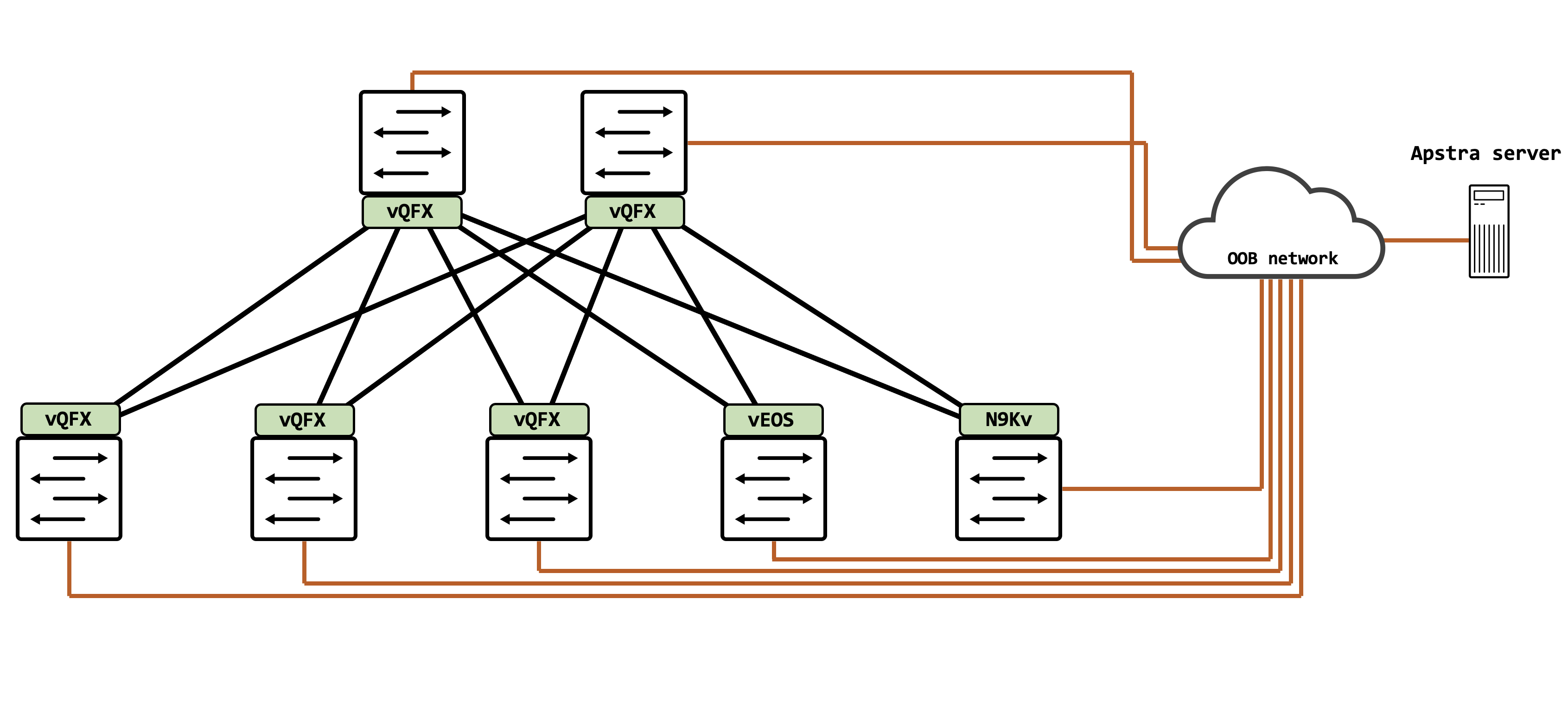
Our topology is the same one we used for Part I of this series. We’re going to be focusing on just the vQFX devices and leave out the Arista vEOS and Cisco N9Kv for now (multivendor via Apstra will be a later post).

Designing a data center rack

Our reference for this entire process is based on Apstra 4.1.0.

Let’s go back to the workflow we’d described in the first post:

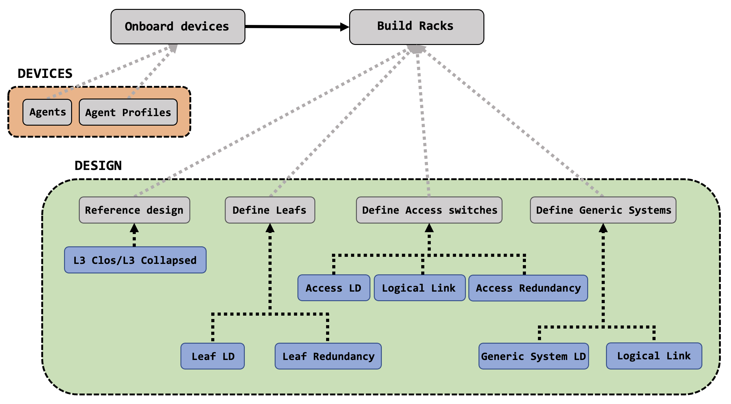
This is what we’re going to detail out here, and understand various components involved in building a rack.

Agents and Agent Profiles

To take action on any device (or collect data from any device), the device must first be known to the system (Apstra, in this case) - it must be a part of the inventory. In Apstra, this is facilitated by something called as ‘Agents’.

Agents can be of two types:

1. On-box - these are agents that are installed directly on the network device itself (applicable only if supported by the network operating system).
2. Off-box - these are agents installed on the Apstra server, as a container, for a particular network device.

A complete compatibility list (what network operating system supports what type of agent) is available in the official Apstra documentation, found here. Navigate to the ‘User Guide’.

Juniper supports only the off-box agent as of Apstra 4.1.0, and detailed instructions regarding the initial configuration required for the off-box agent to be installed can be found here for Apstra 4.1.

If you don’t want to read the guide, here’s a quick summary: a super-user that Apstra will use to login to the system, ssh and netconf over ssh, and finally reachability to the network device from Apstra.

{master:0}[edit]
root@vqfx# show system login 
user aninchat {
    uid 2000;
    class super-user;
    authentication {
        encrypted-password "$6$CR8rOdvC$fZiYRGtALKZNGU1hWCyoNg5fqxqyJlANacEwEfRPHLawUWzzpMLdMw1NpR5Z3//hPckVZbTjYFkCHPBdaKzxo."; ## SECRET-DATA
    }
}

{master:0}[edit]
root@vqfx# show system services 
ssh {
    root-login allow;
}
netconf {
    ssh;
}

As part of the device discovery, some basic parameters are needed, which are a part of constructing the Agent itself - this includes the platform (junos/eos/nxos), the IP address to reach the device and the username/password for logging into the device.

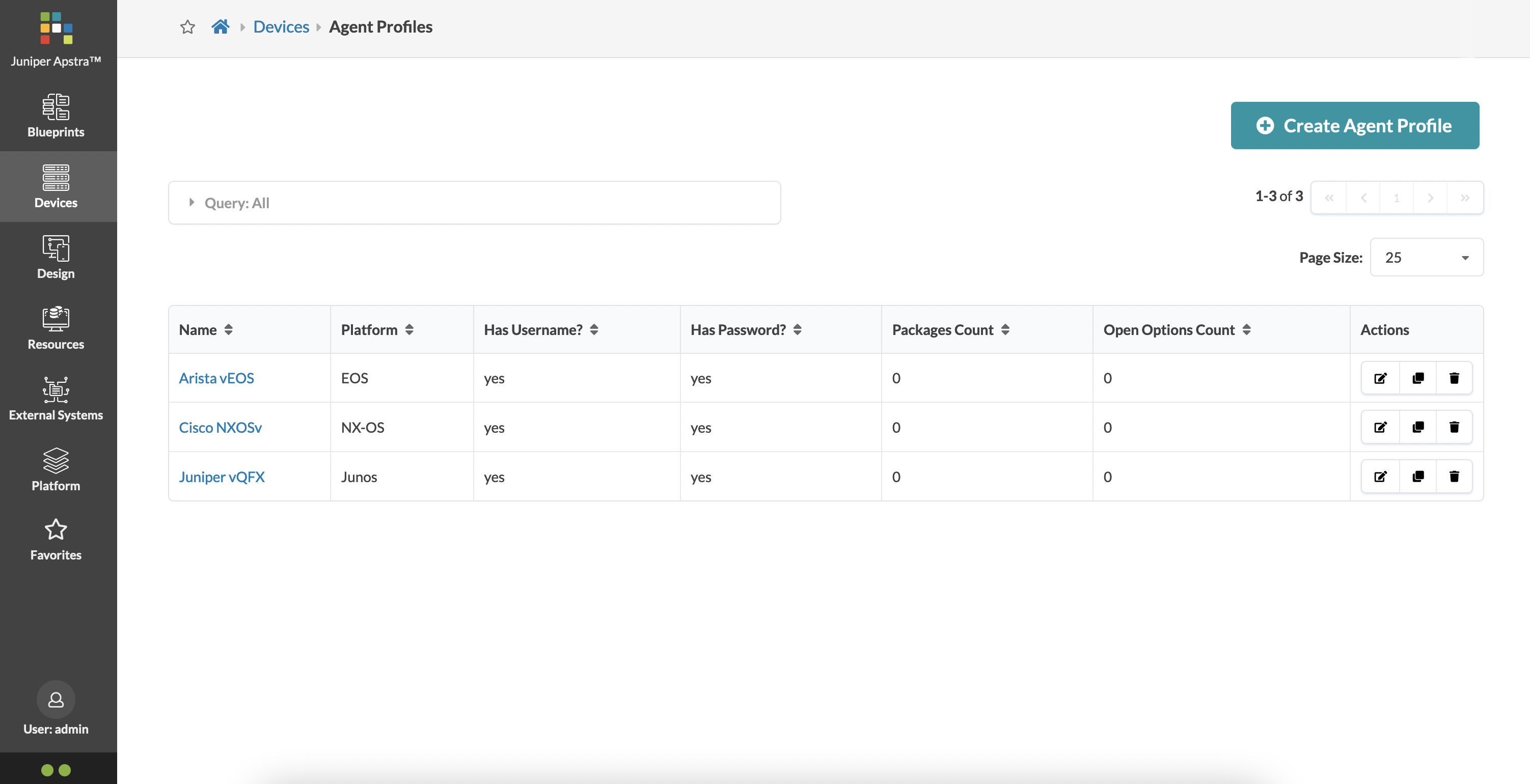
As you can imagine, this can get pretty tedious if you have to choose the platform and type in the username/password every single time for every new device that needs to be onboarded. This is where Agent Profiles are useful - you can create a profile for a specific type of device and just use the profile whenever that type of network device needs to be onboarded.

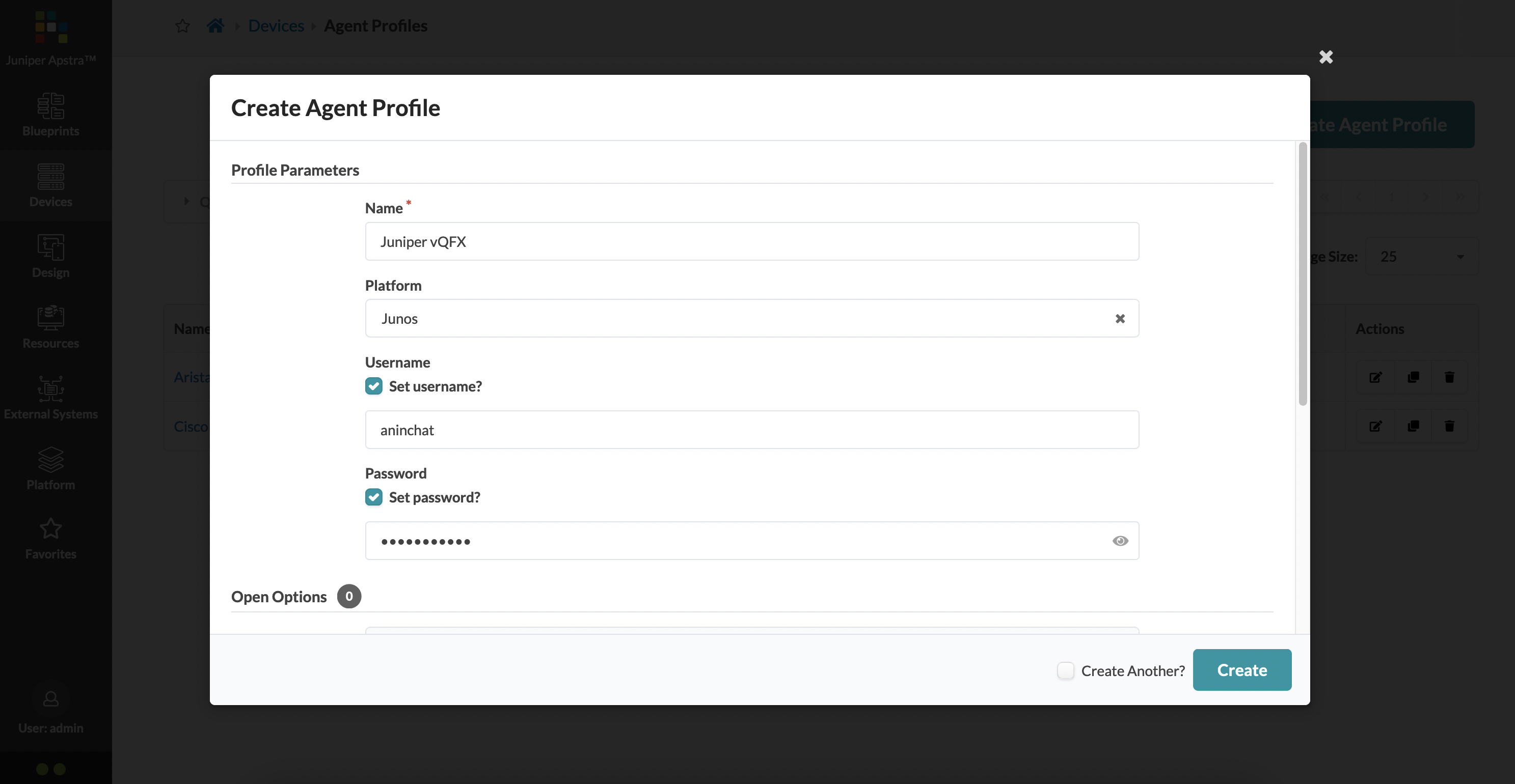
As an example, let’s create an Agent Profile for my vQFX devices that need to be onboarded:

You can see that I also have similar profiles created for Arista vEOS and Cisco N9Kv:

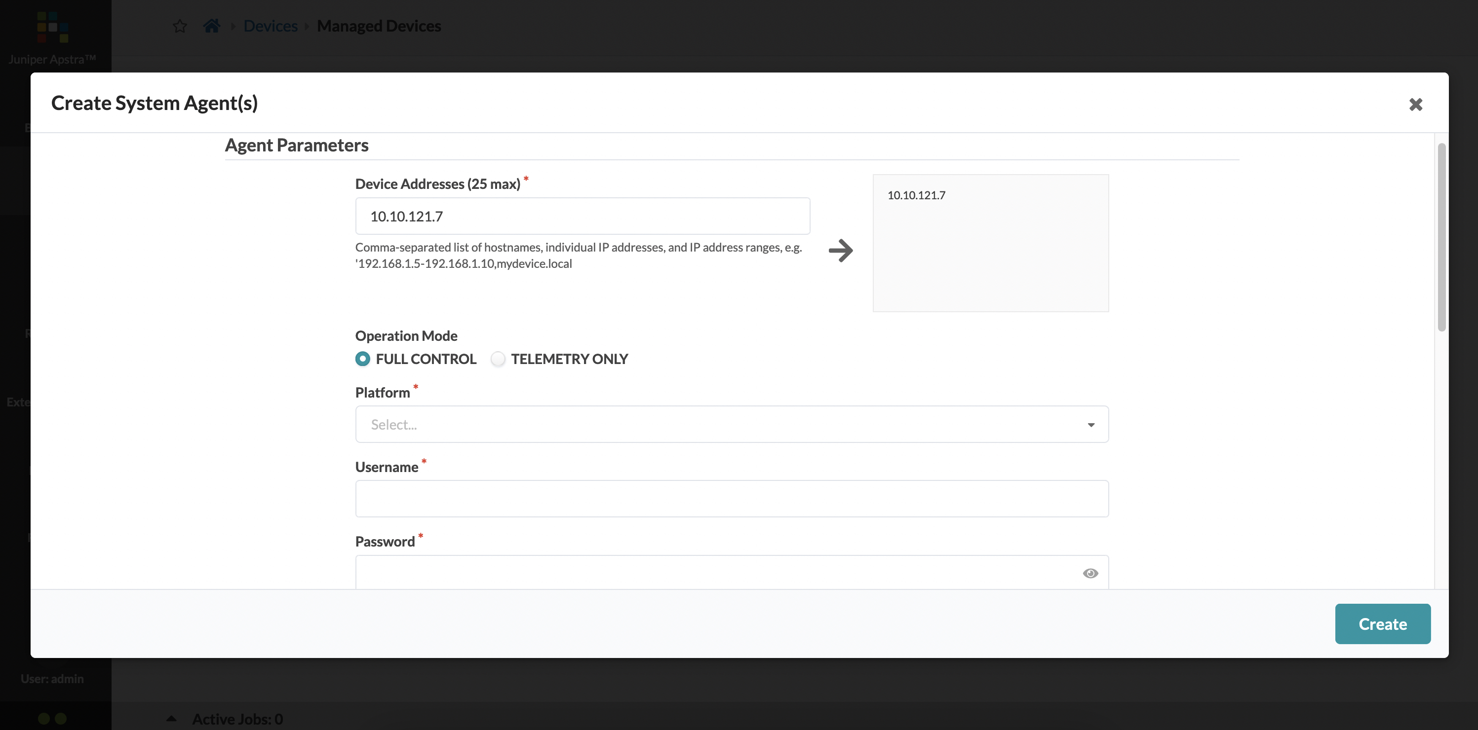
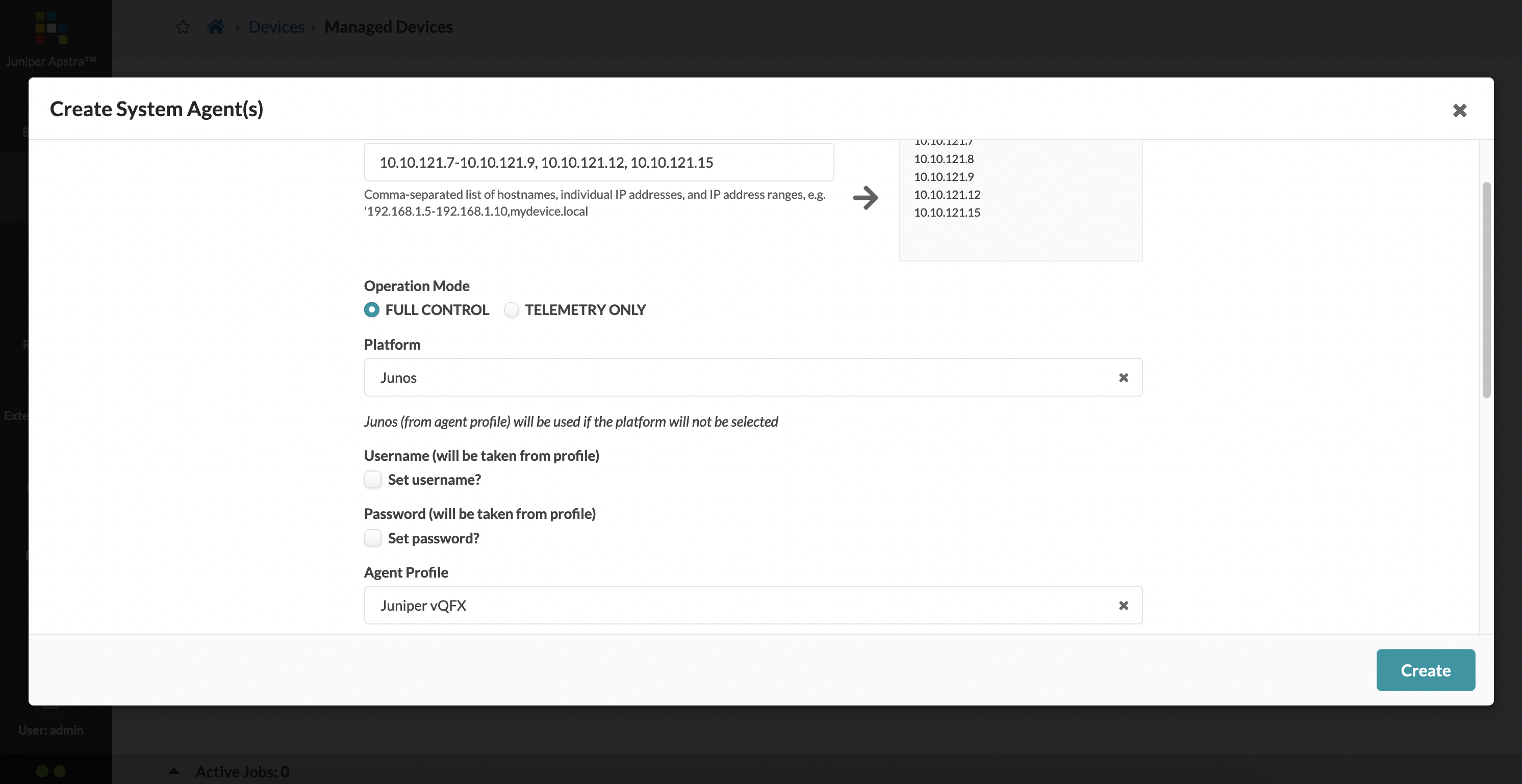
Now, I can type in the IP addresses of the devices I want to onboard (my two vQFX spines, and three vQFX leafs, in this case) and choose the vQFX profile.

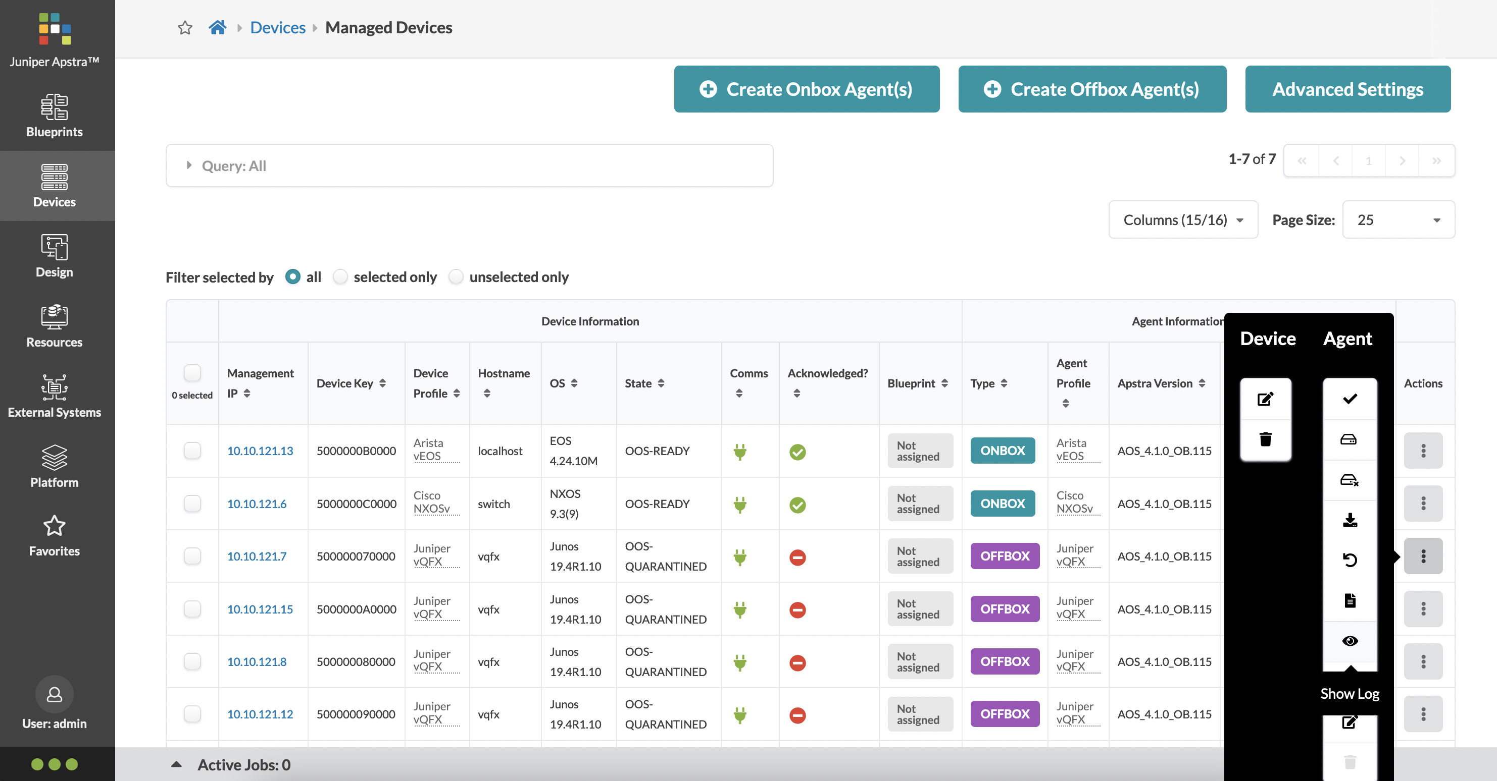
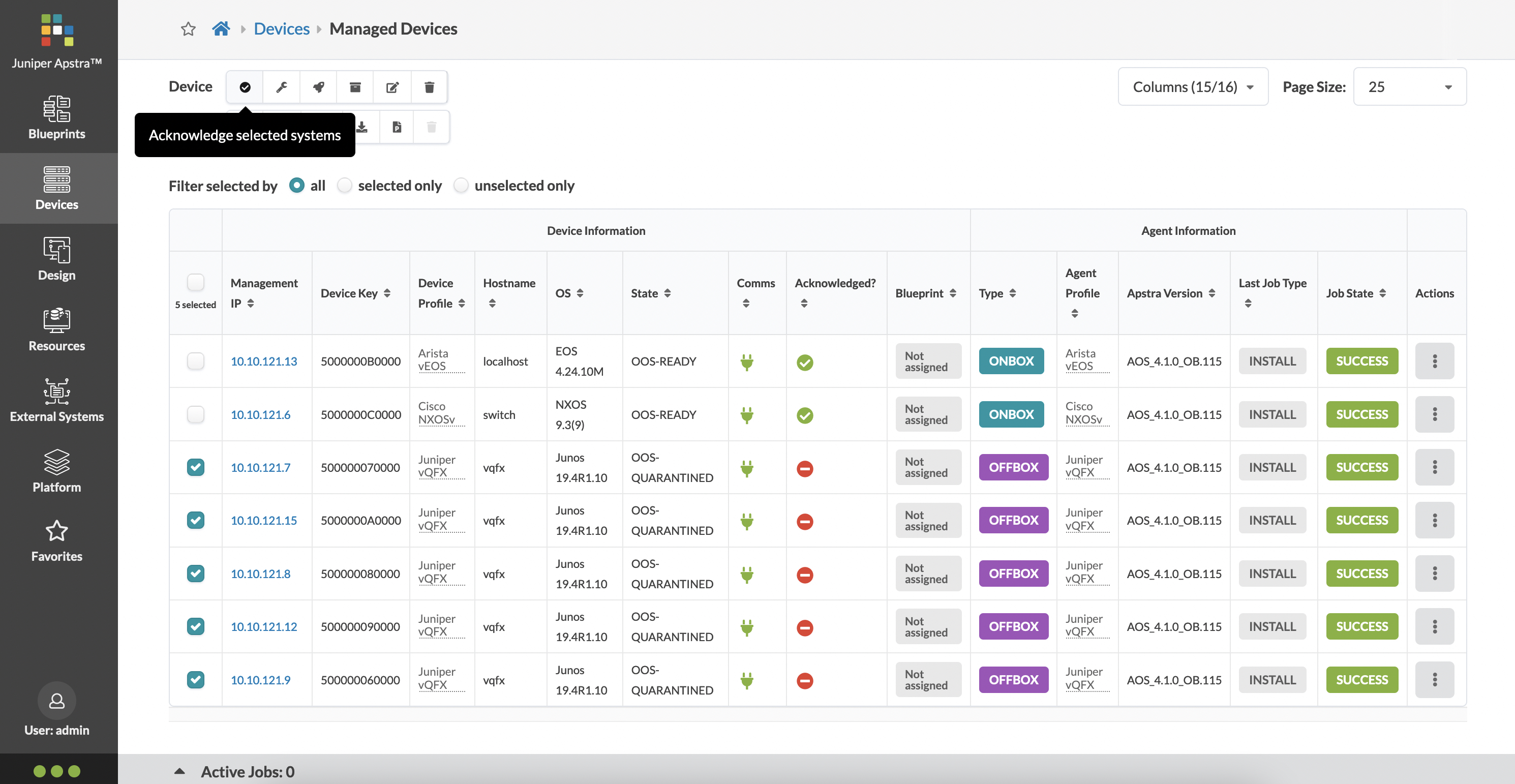
These devices are now listed under ‘Managed Devices’ under the main ‘Devices’ tab. While Apstra makes contact with the devices that need to be onboarded, and collect data that it needs to onboard it, you can view the logs for any device that is being onboarded (or was onboarded already).

Just click on the button with the three dots (extreme right of each device row), and you get a set of actions available to you for that particular device. One of these actions is ‘Show Log’.

The logs from a successful onboard of a vQFX device looks something like this:

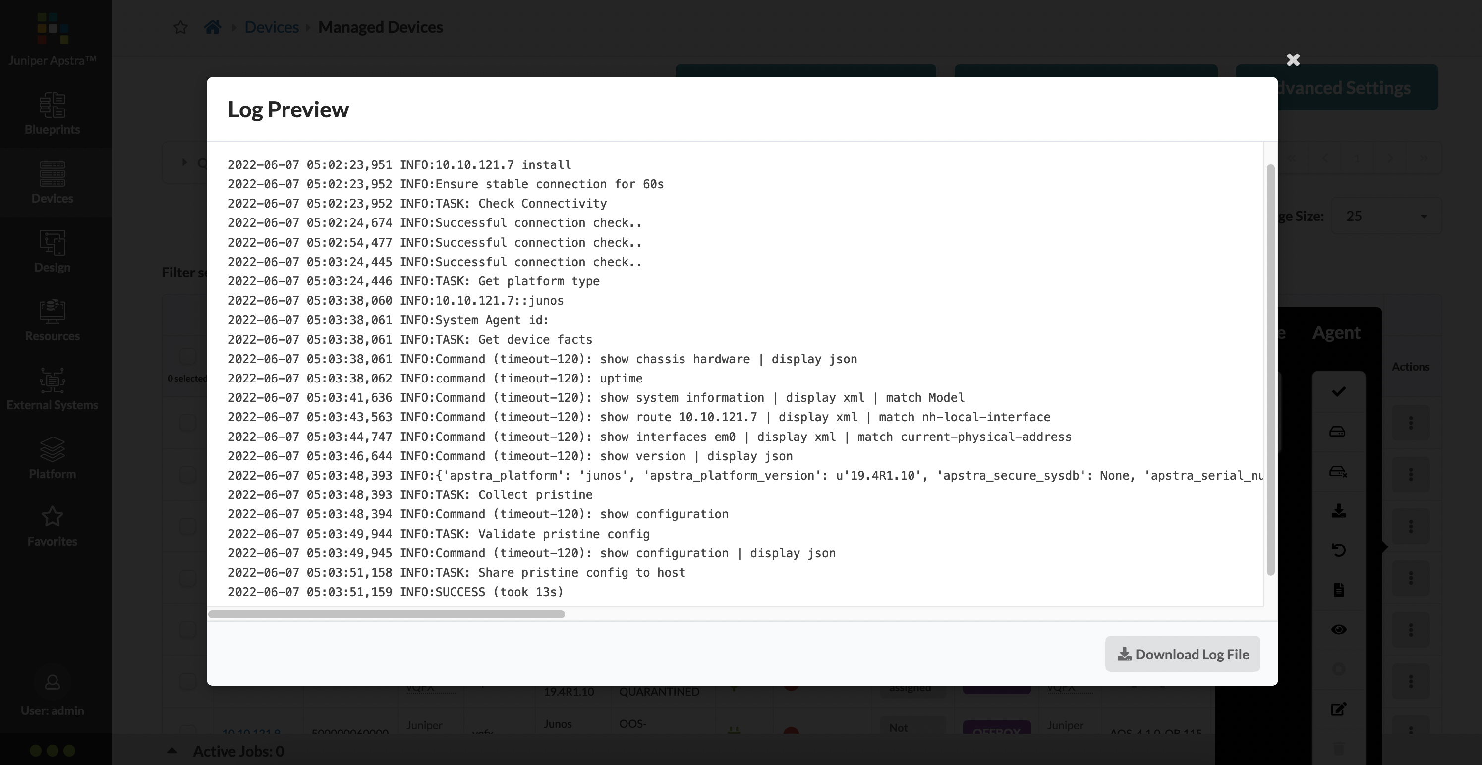
As part of the process, Apstra collects the configuration from the device and stores it as the pristine configuration - this is the baseline configuration without any services and features added to the device, apart from what was needed to get the device onboarded into Apstra. The Apstra state for the device at this point is called ‘OOS-QUARANTINED’ where ‘OOS’ stands for ‘Out Of Service’.

The entire device lifecycle can be found here. Once a device is onboarded, it needs to be explicitly acknowledged by Apstra - this acknowledgment kicks off the ‘Discovery 1’ process where LLDP is enabled on all interfaces. You can acknowledge a device by selecting the device (or selecting a subset of devices) and clicking on the ‘acknowledge selected systems’ button, and a subsequent confirmation:

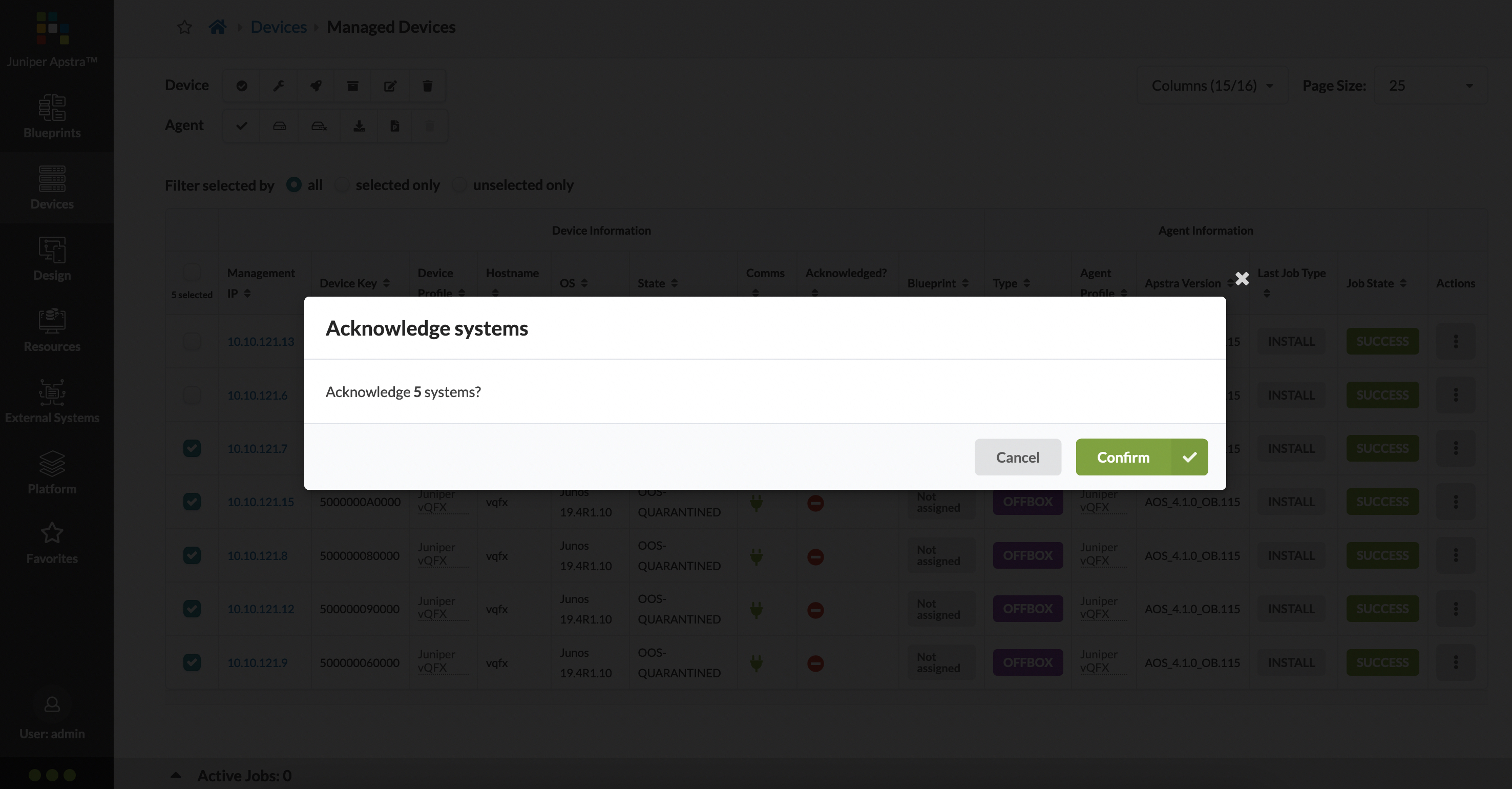
At this point, connected devices should see each other as LLDP neighbors. The Apstra state for the device moves from ‘OOS-QUARANTINED’ to ‘OOS-READY’ which essentially implies that the device is out of service, but it is ready and can now be added into a blueprint.

Logical Devices

Logical Devices, as the name suggests, are just a logical or abstracted representation of your network device. The important thing to remember is that this is not vendor specific at all - you’re not choosing Cisco or Arista or Juniper with a logical device. You’re simply stating that you’d like a device that has, for example, 24x10G ports, with 4x100G uplinks. Or whatever other speed/port combination you’re looking for.

A logical device also allows you to specify what kind of devices these ports can be connected to and used for - again, for example, you’d like your 4x100G uplinks to be used for connections to a spine, and your 24x10G ports as connections to servers.

Logical devices can be found under ‘Design’. There are numerous logical devices that are already pre-built, covering a large range of existing (and supported) network devices from different vendors such as Cisco, Arista and Juniper.

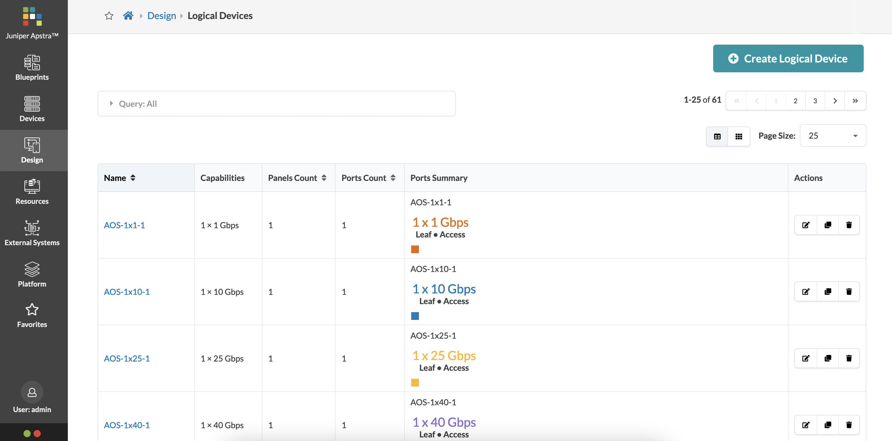
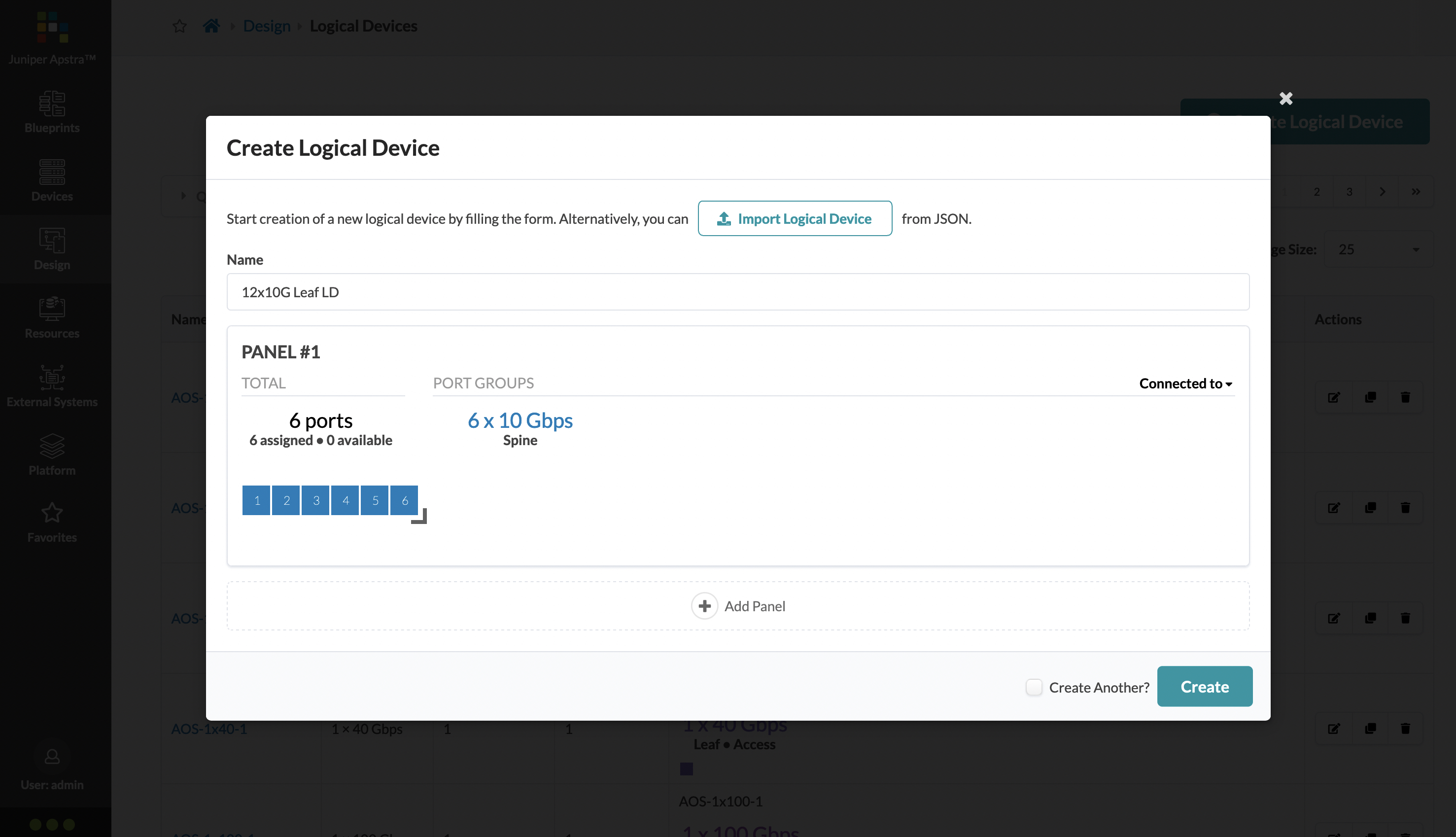
We’re going to create two new logical devices to go through the workflow: one for a vQFX leaf, and another for a vQFX spine. We’re also going to be specific with what ports can connect to what network devices.

We’re going to have 6 ports available on the leaf (10G each) to connect to spines:

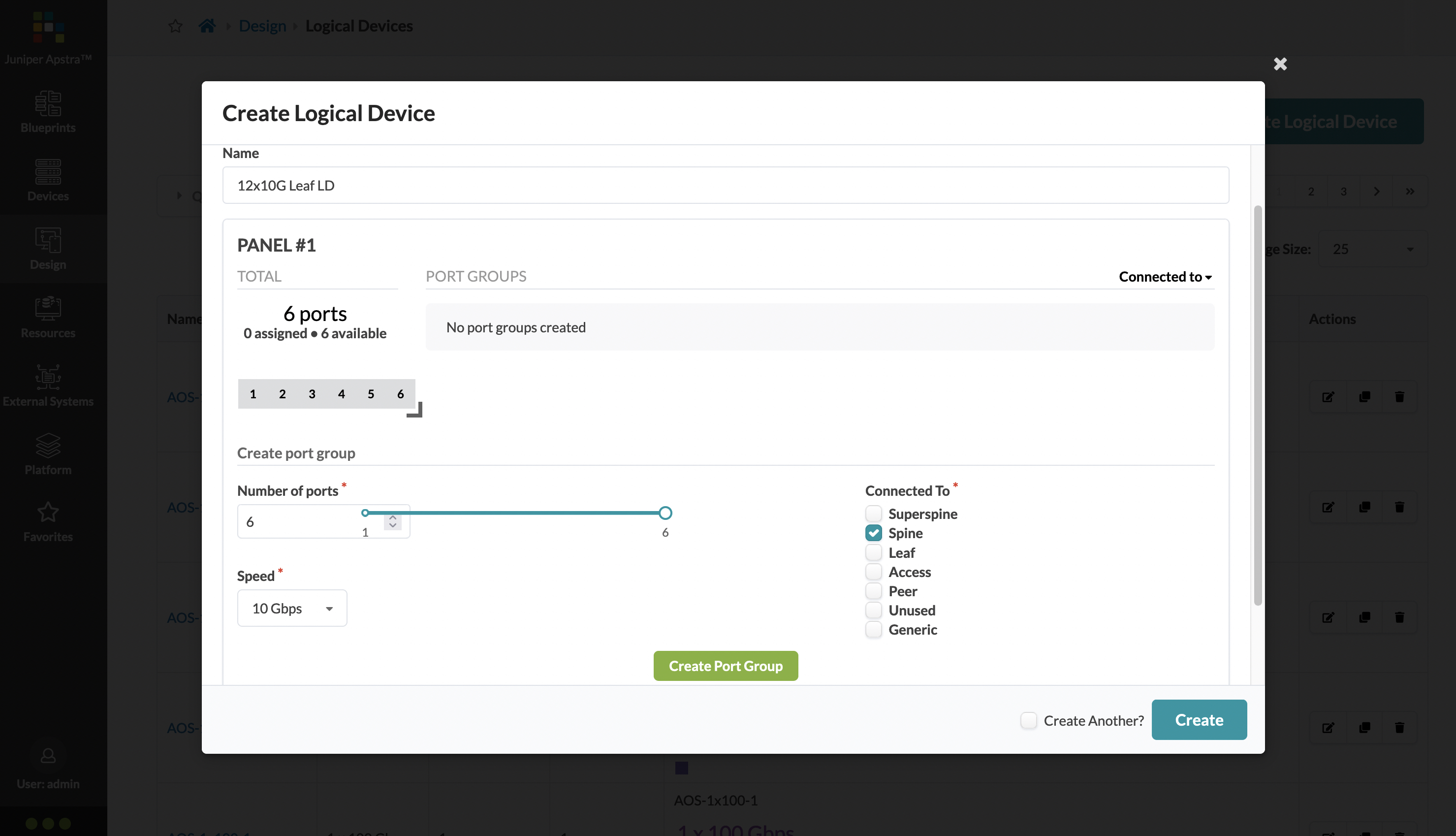
Click on the ‘Create Port Group’ option to create a port group for these 6x10G ports.

You can continue to add more ports by dragging the port group further. We’re going to add another 6 ports that can be used to connect to the hosts. Hosts can be selected as ‘Generic’:

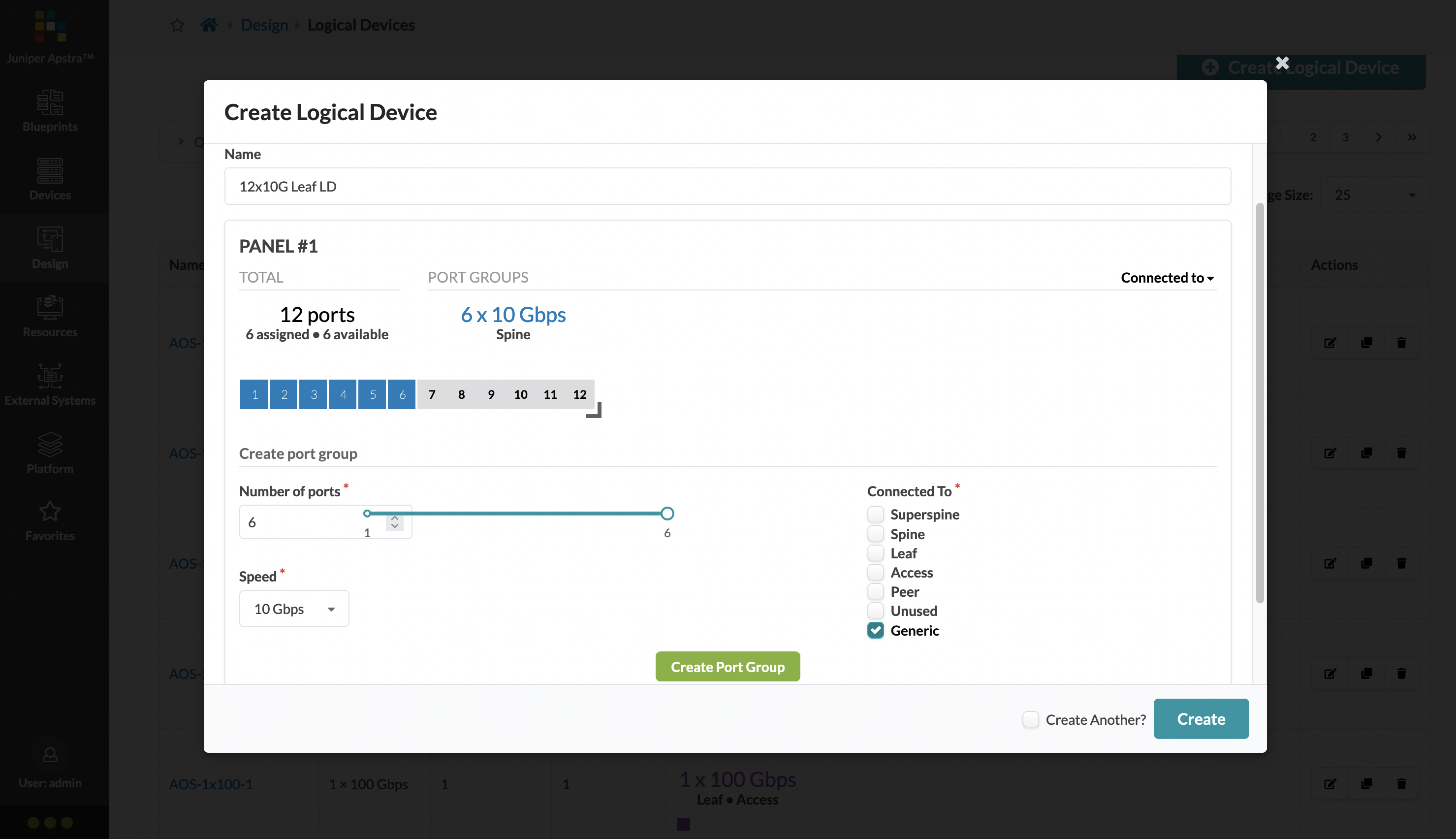
You should now have a 12x10G vQFX logical device:

Click on ‘Create’ to create this logical device. We’re going to do the same thing for our vQFX spines, but all ports are going to be marked as connected to leafs.

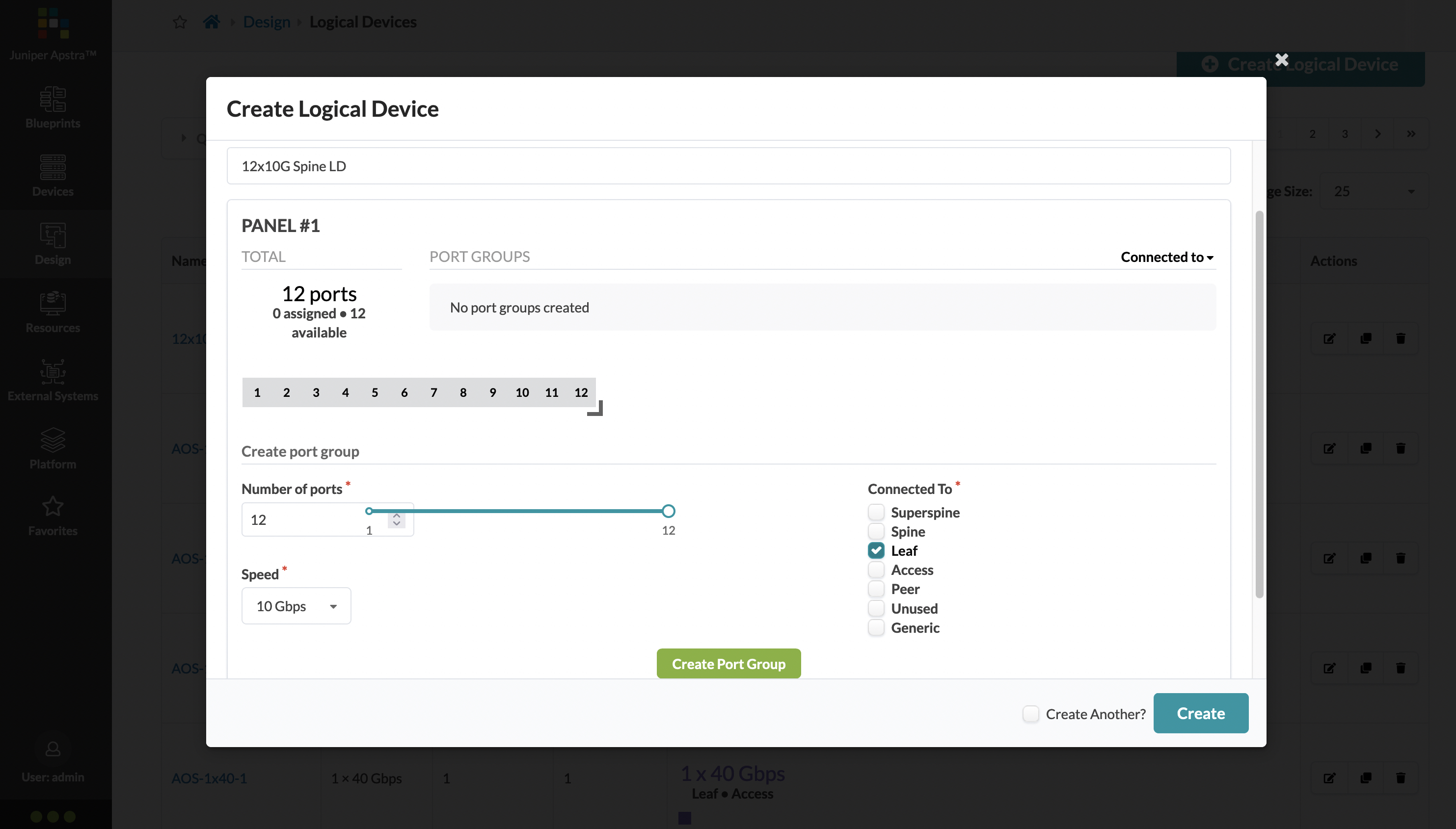
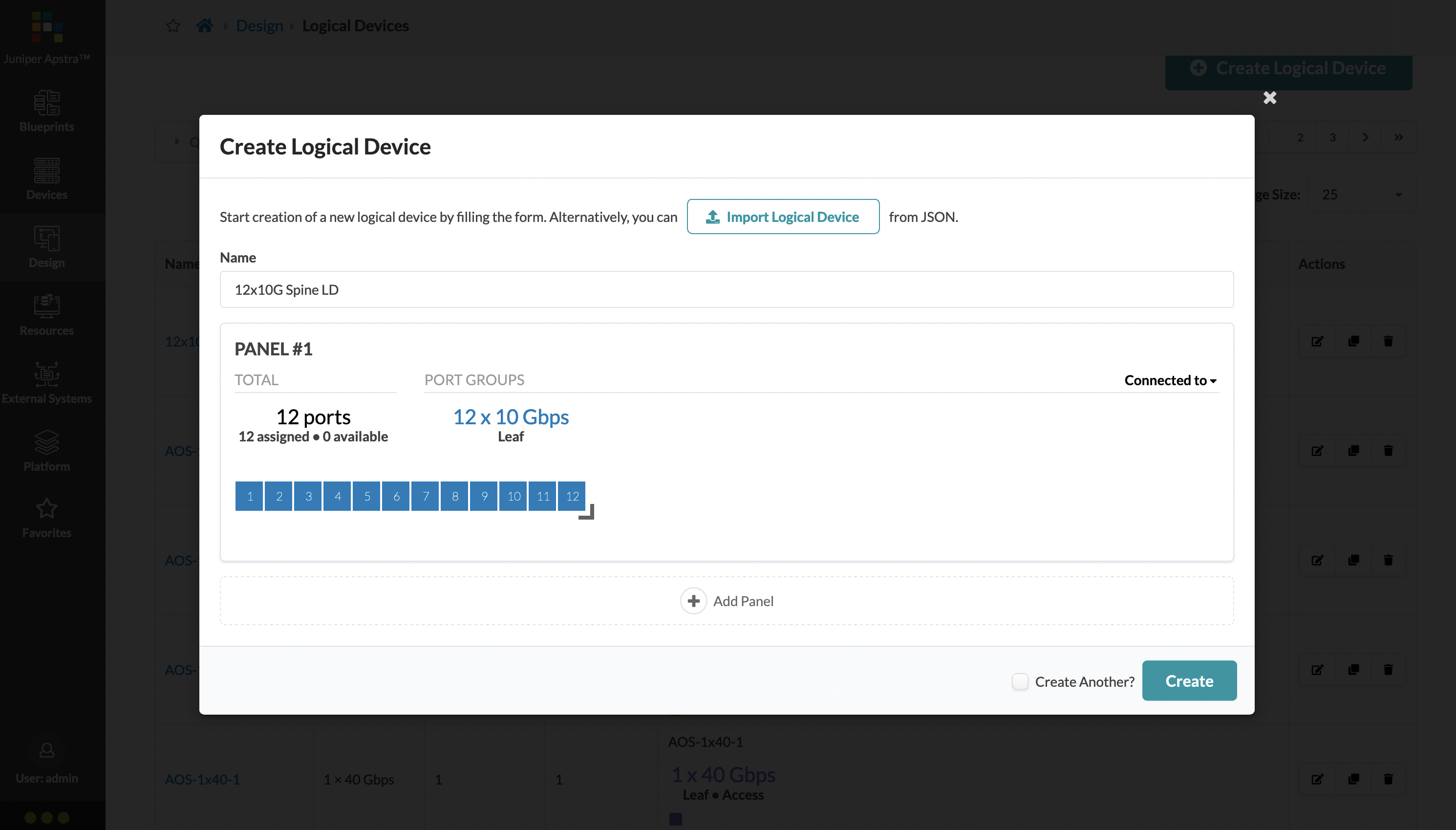
Create the port group, and click on create just like before to build this vQFX spine logical device:

Device Profiles

Device Profiles are where the actual hardware is defined. This includes (among other things):

• what kind of vendor specific model the hardware is (PID)
• the network operating system
• what versions to match on (based on a regular expression)
• CPU and RAM on the device
• the kind of ASIC it supports
• CoPP support
• interfaces, the kind of connector type for it, and the naming convention

For vQFX (as well as vEOS and N9Kv), a device profile already exists, so we’re not going to create a new one. But I’d still like to walk you through some of these options to show you how it can be done, particularly how the ports are defined via “transformations”.

Device Profiles can be found under ‘Devices’. The main page for this lists out all of the available device profiles, with a search bar to filter as you wish.

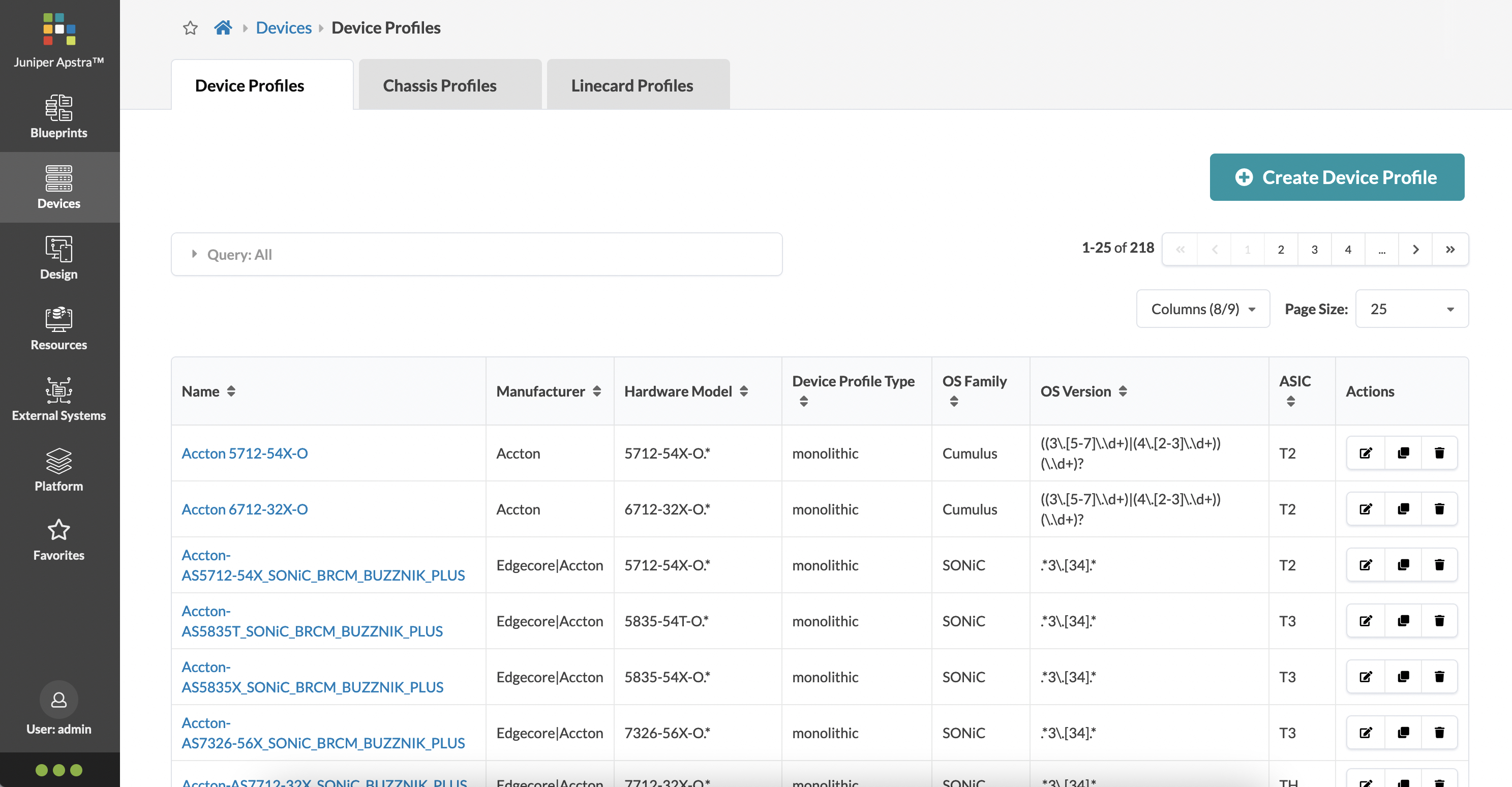
If you’d like to create a new profile, you’re met with the following page and options:

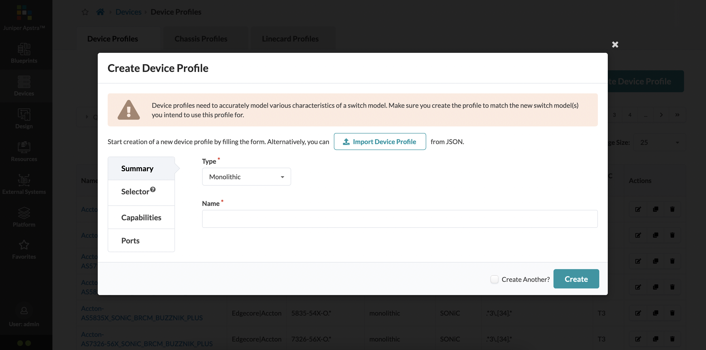
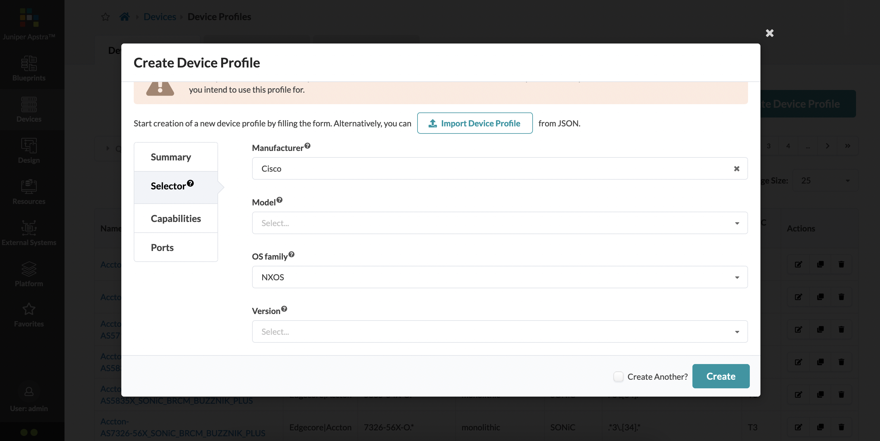
The selector option lets you specific more vendor specific information:

I want to focus on the ‘Ports’ section for a little bit, as that is very interesting. Here, you’re greeted with a famiilar looking UI (this is similar to how we created logical devices). By default, one panel is present which is what you’d have for a non-modular network device. Considering our vQFX example, this panel should have 12 ports:

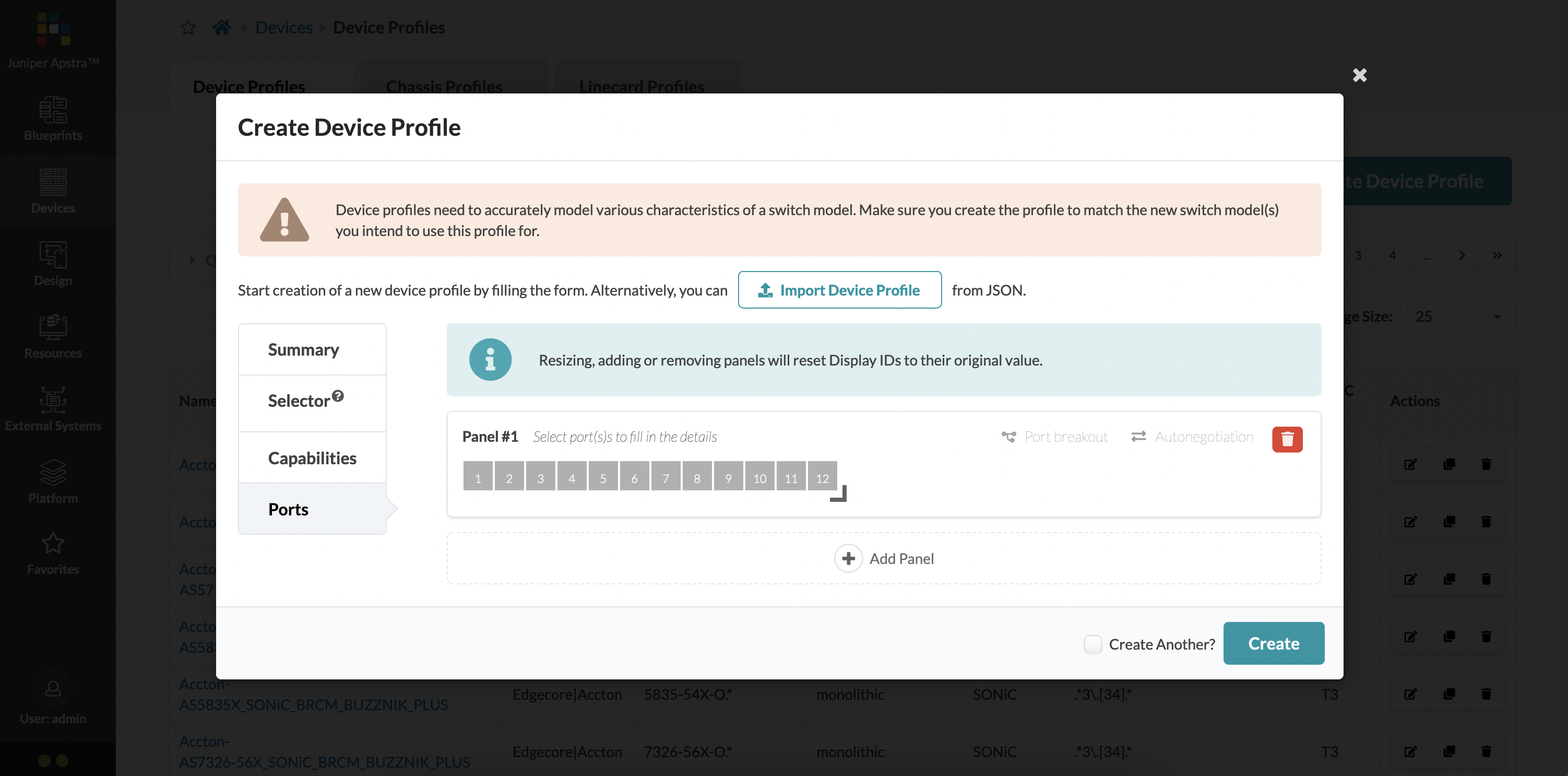
You can now select a port, a subset of ports or all the ports to associate properties against them, like the connector type (SFP, QSFP and so on). For example, I have selected port 1 (by simply clicking on it):

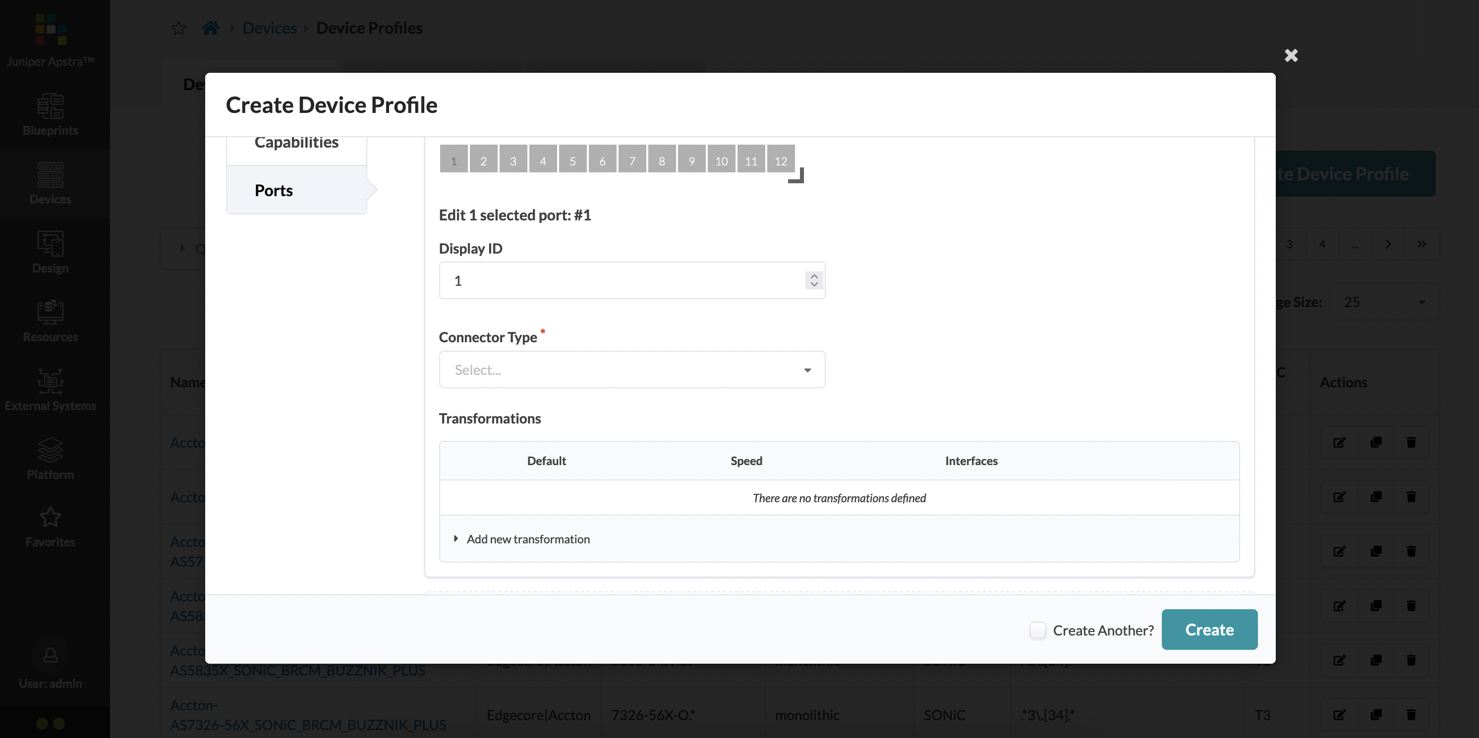
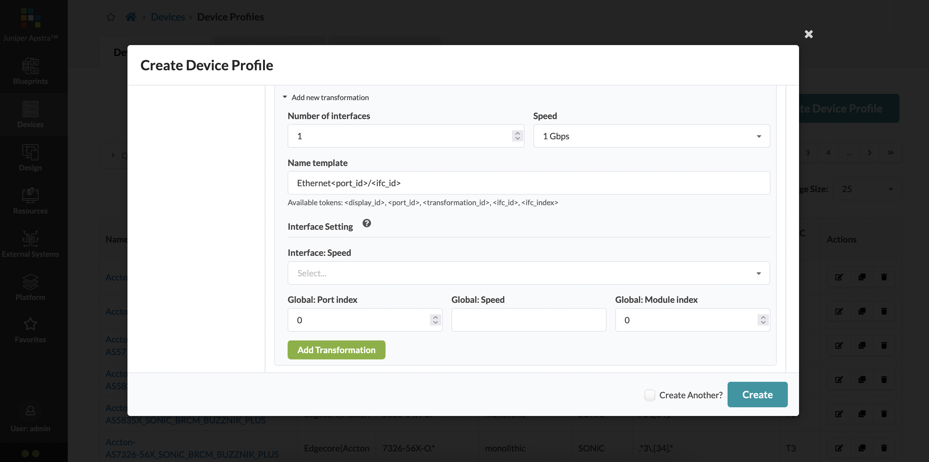
You also need to associate a “transformation” against the port. This is how the interface naming is actually generated (which, as you can imagine, can be vastly different from vendor to vendor), as well as the speed of the interface. Clicking on ‘Add new transformation’ lets you do this.

Before we move on from this, I’d like to show you the pre-built vQFX device profile:

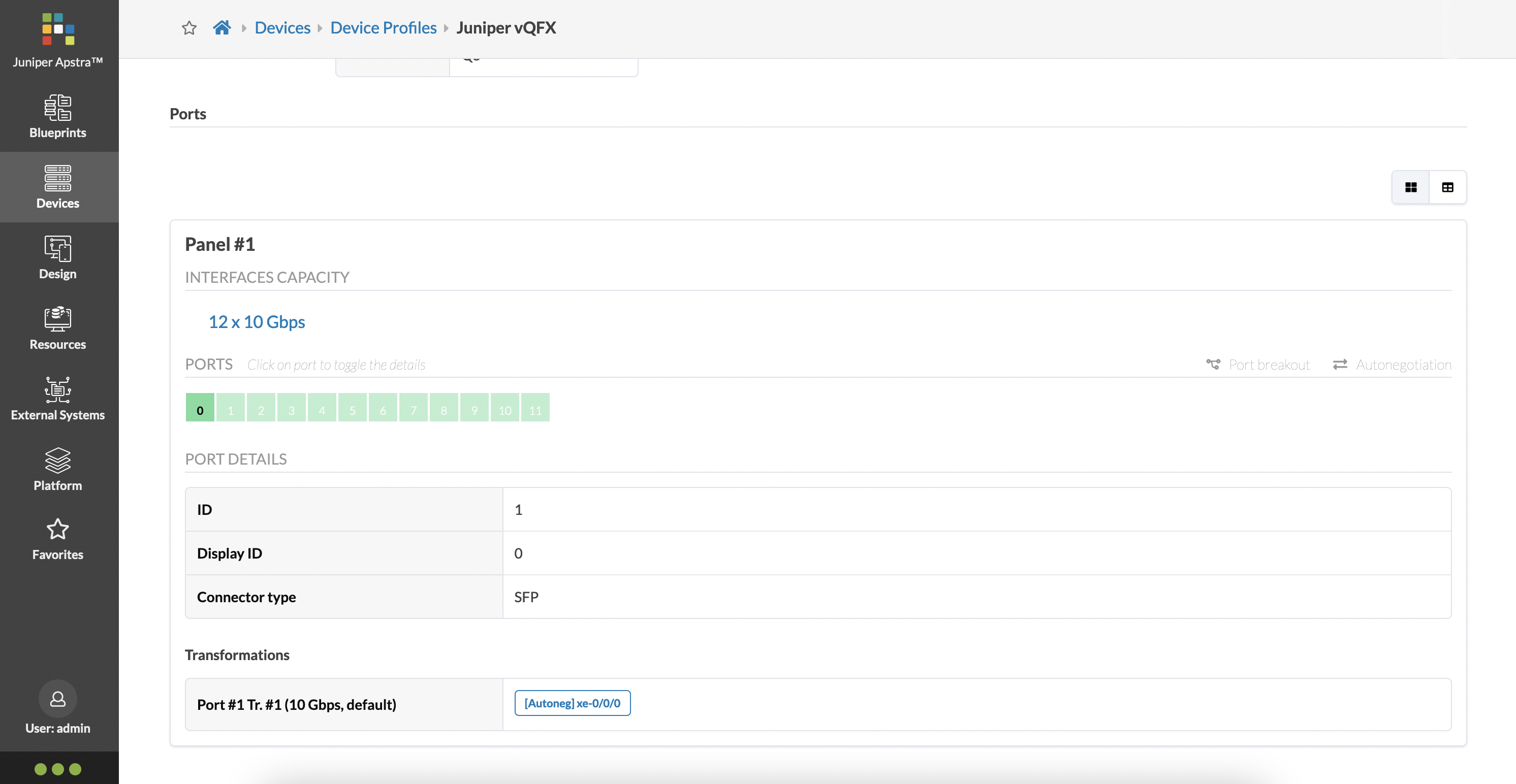
These are 12x10G ports, with the transformation defining the interface naming as xe-0/0/0 for port 1 and so on, which is what we expect.

The transformations do more than just this - these are extremely crucial for defining breakouts as well. You can simply have multiple transformations defined which allows you to create port breakouts - for example, let’s say the actual vendor hardware you buy allows for a 40G port to be split into 4x10G ports. How would you deal with this in Apstra? You would simply create two transformations - one for the 4x10G ports and another for the 1x40G port.

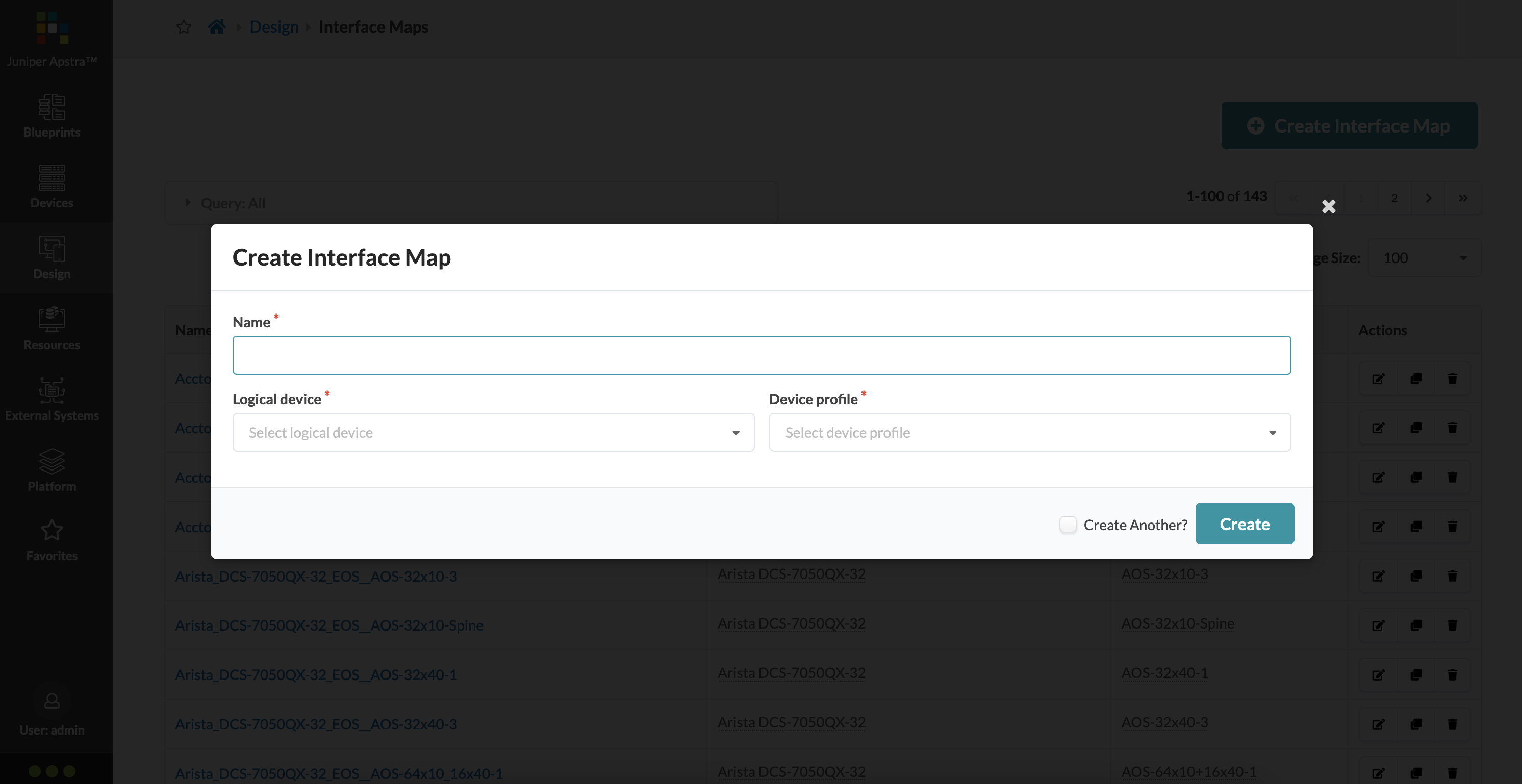
Interface Maps

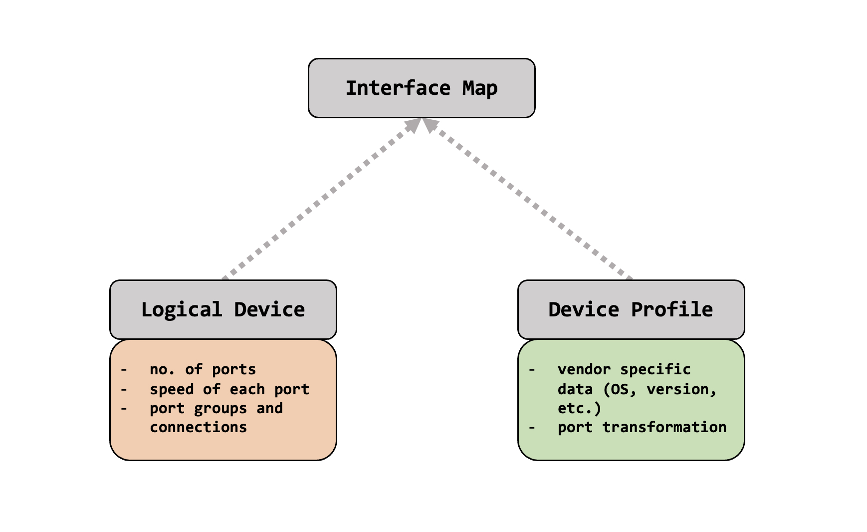
Interface Maps are fairly straightforward, but extremely important. A logical device and a device profile feed into it, and are used to create an interface map. This is where your logical abstraction of a device, and it’s hardware specific information all comes together to form an actual deployable network device in your blueprint (which we’ll talk about in the next post).

From the UI, this is found under ‘Design’ again. Like I said, an interface map just takes in two feeds - a logical device, and a device profile.

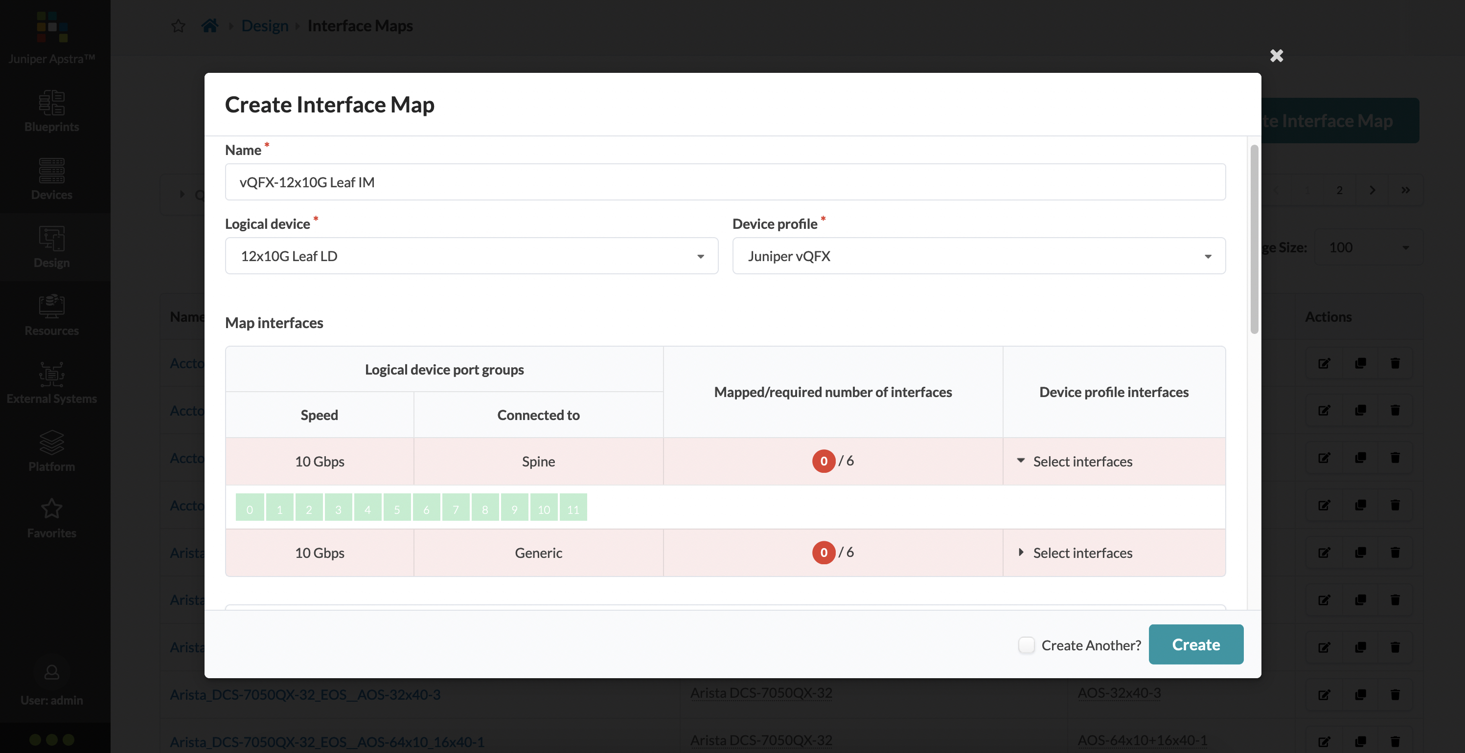
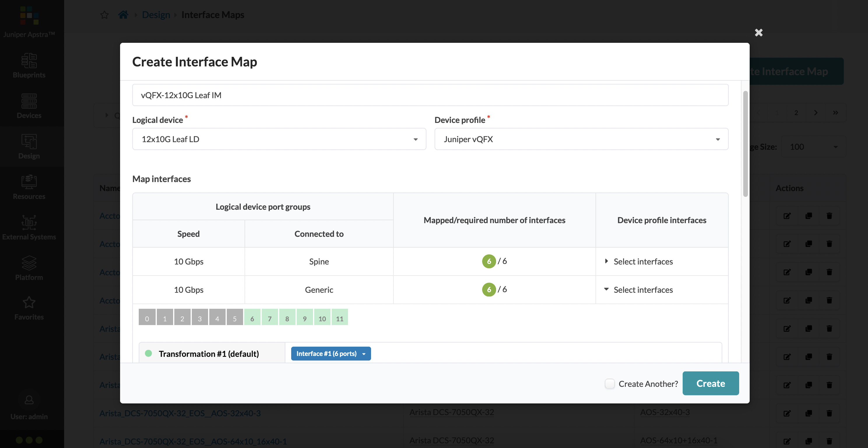
For our case, we’re going to create two interface maps - one for the vQFX leaf and another for the vQFX spine. Starting with the leaf, we have our leaf logical device and the vQFX device profile as the input. Once this is done, there is some additional selection that needed - this is the port selection for the port groups that were created within the logical device:

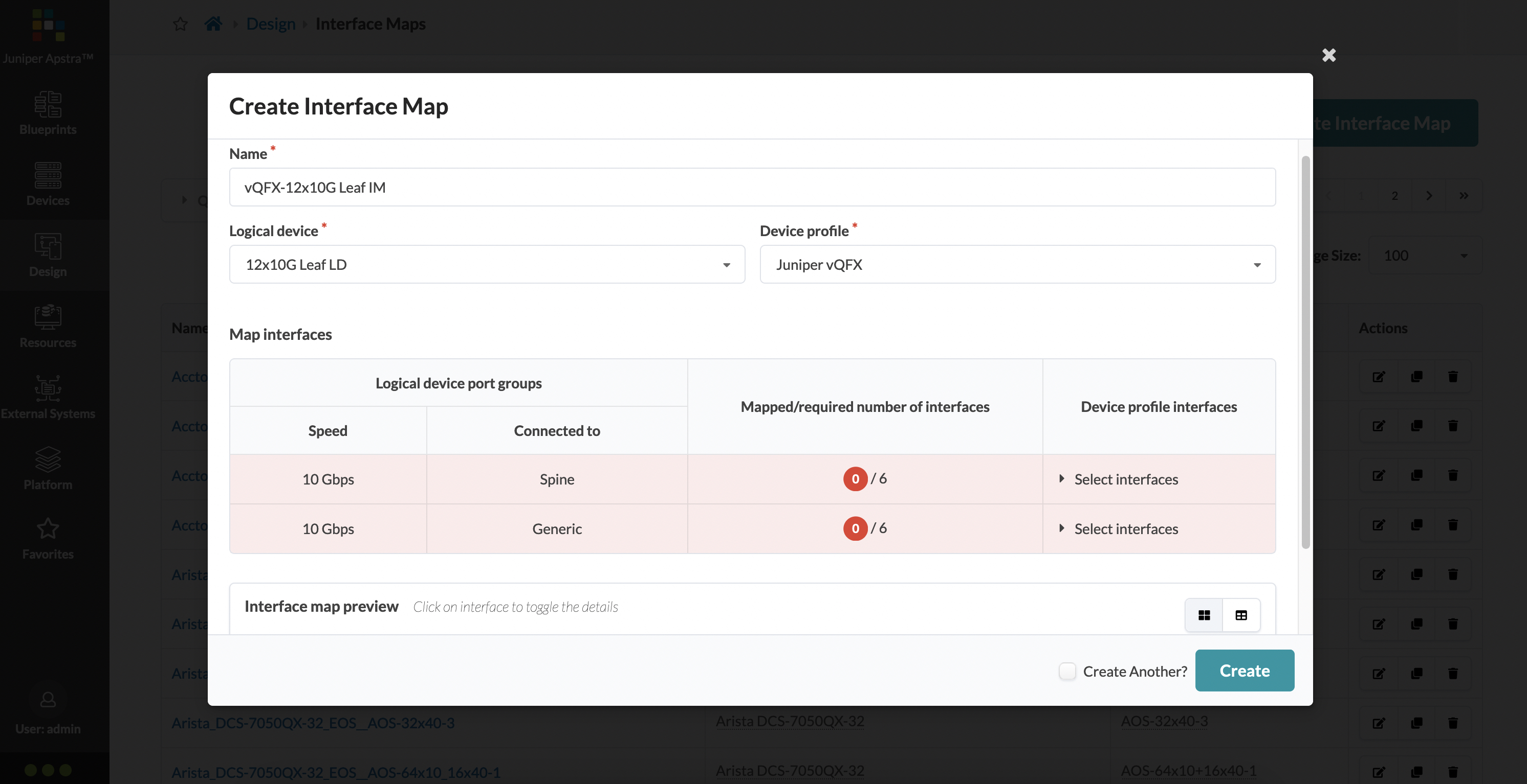
The ‘Select Interface’ is kind of a drop down, which when clicked, lists all the available ports that can be selected (and mapped using the device profile) for that port group.

This can be a little confusing, since it might seem like we did this exercise while creating a logical device as well, but think of it as this way - with the logical device, you’re only defining the number of ports, their speeds, and what they are allowed to be connected to. In the interface map (and using the device profile), you’re actually selecting which ports can do what and mapping them to a vendors standard naming convention (using a transformation that was defined in the device profile) for that kind of port.

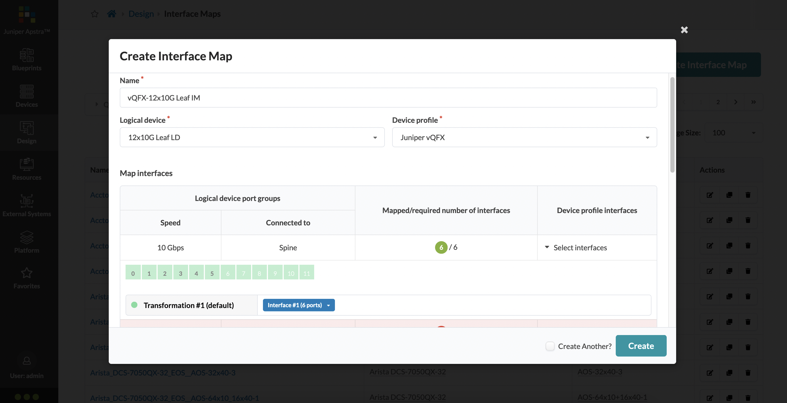
So, in our case, I’d like the first 6 ports to be available as my spine connections, and use transformation #1 which was the default transformation present in the pre-built vQFX device profile. Let’s select those:

The remaining 6 ports are now chosen for my host/server connections:

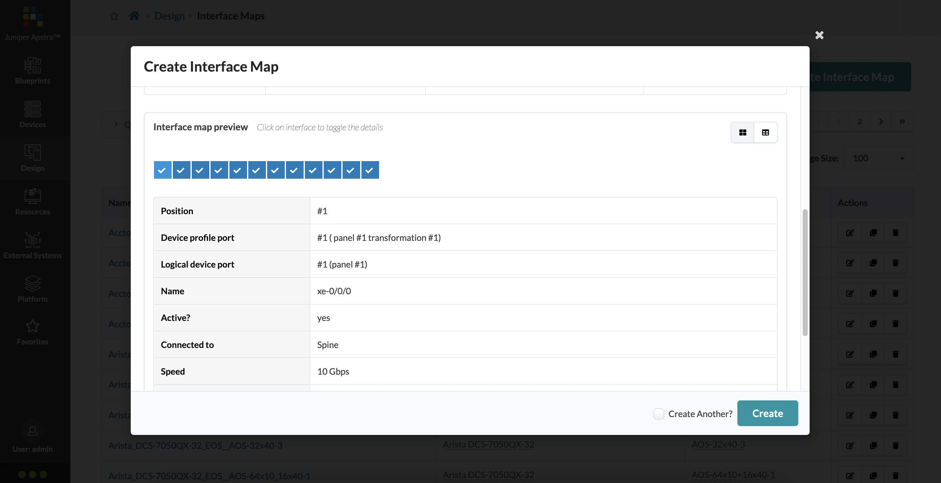
Finally, as a confirmation, if you scroll down a bit during the interface map creation, you can select any port to see a summary of what it would look like when actually deployed. I’ve selected port 1, which tells me it is port #1 of panel #1, and it is named xe-0/0/0.

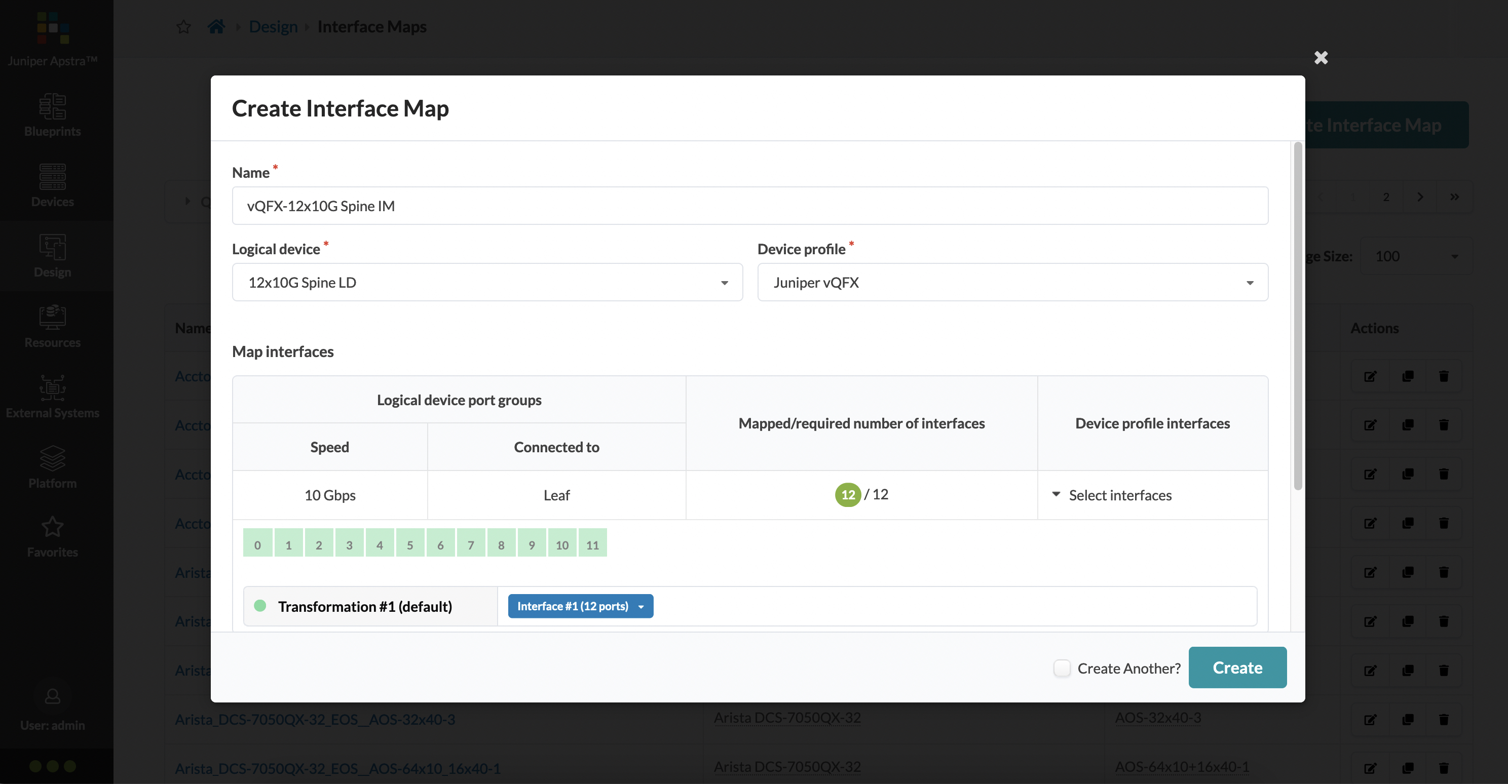
For our spine interface map, a similar process can be followed. In this case, there is just one port group with all 12 ports, and we select all of them with the same default transformation #1 from the pre-built vQFX device profile.

Putting it all together to build a rack

Well, we’re finally here. We’ve got all our building blocks setup, and it’s time to actually build a data center rack.

Racks are found under ‘Design’ and like everything else, there are several pre-built racks for you. To demonstrate how it’s done, we’re going to build a rack from scratch. Our goal is to build a rack that has one vQFX leaf and two hosts attached to it. It is minimal, and a little unrealistic, but the aim is to largely show you how these different pieces fit together and what the workflow looks like for this.

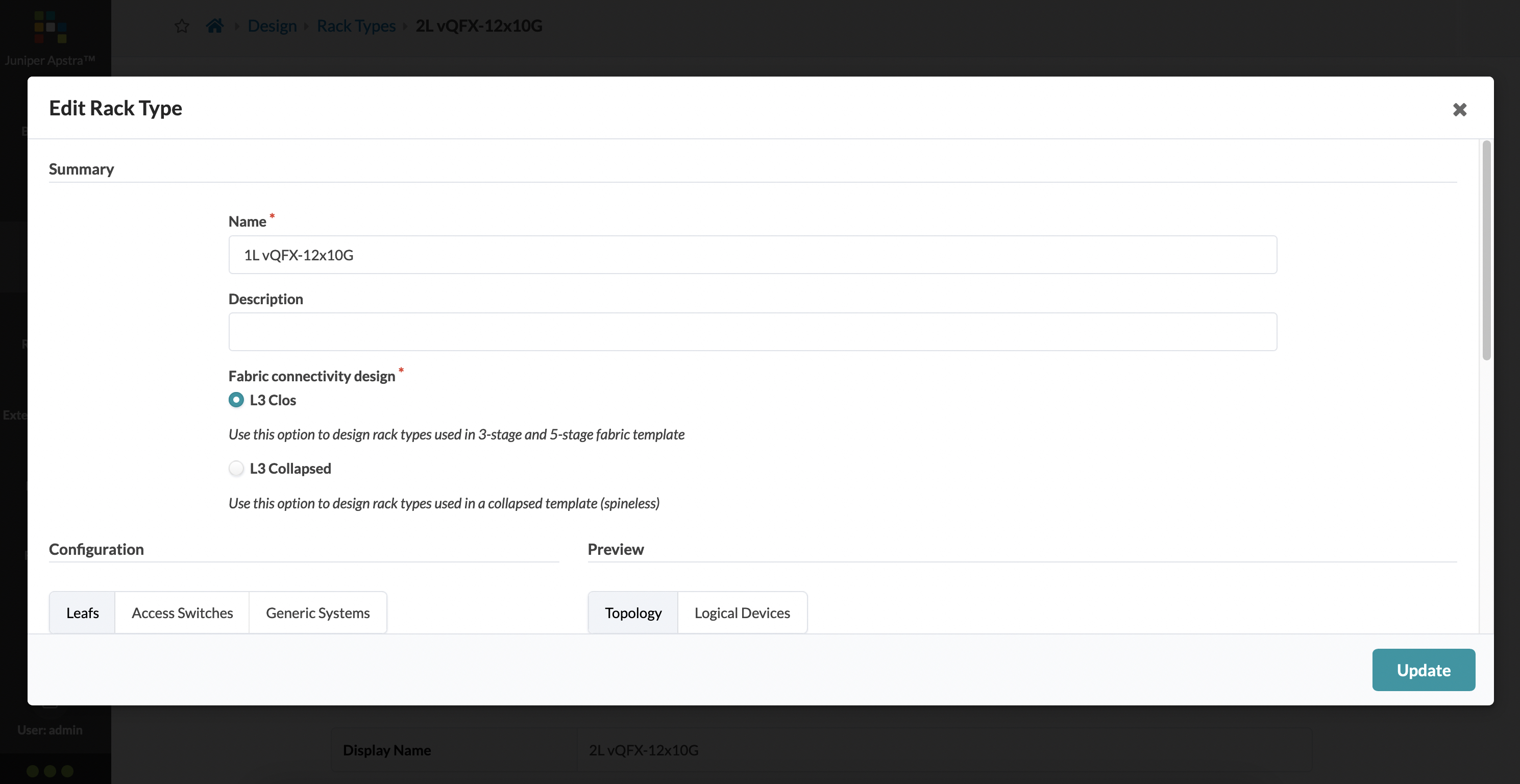
We’re going to give our rack a name - ‘1L vQFX12x10G’, which makes it easy for me to understand that this is a one leaf rack, where the leaf is a vQFX with 12x10G ports. We want to build a 3-stage Clos fabric, so we’re going to choose the ‘L3 Clos’ option. Alternatively, you can choose the ‘L3 Collapsed’ design, where there are no spines.

Now we can move into the configuration of the rack - this is where you define the number of leafs, kind of leafs, how many hosts, if there are any access switches (that sit between the leaf and the hosts)) and so on.

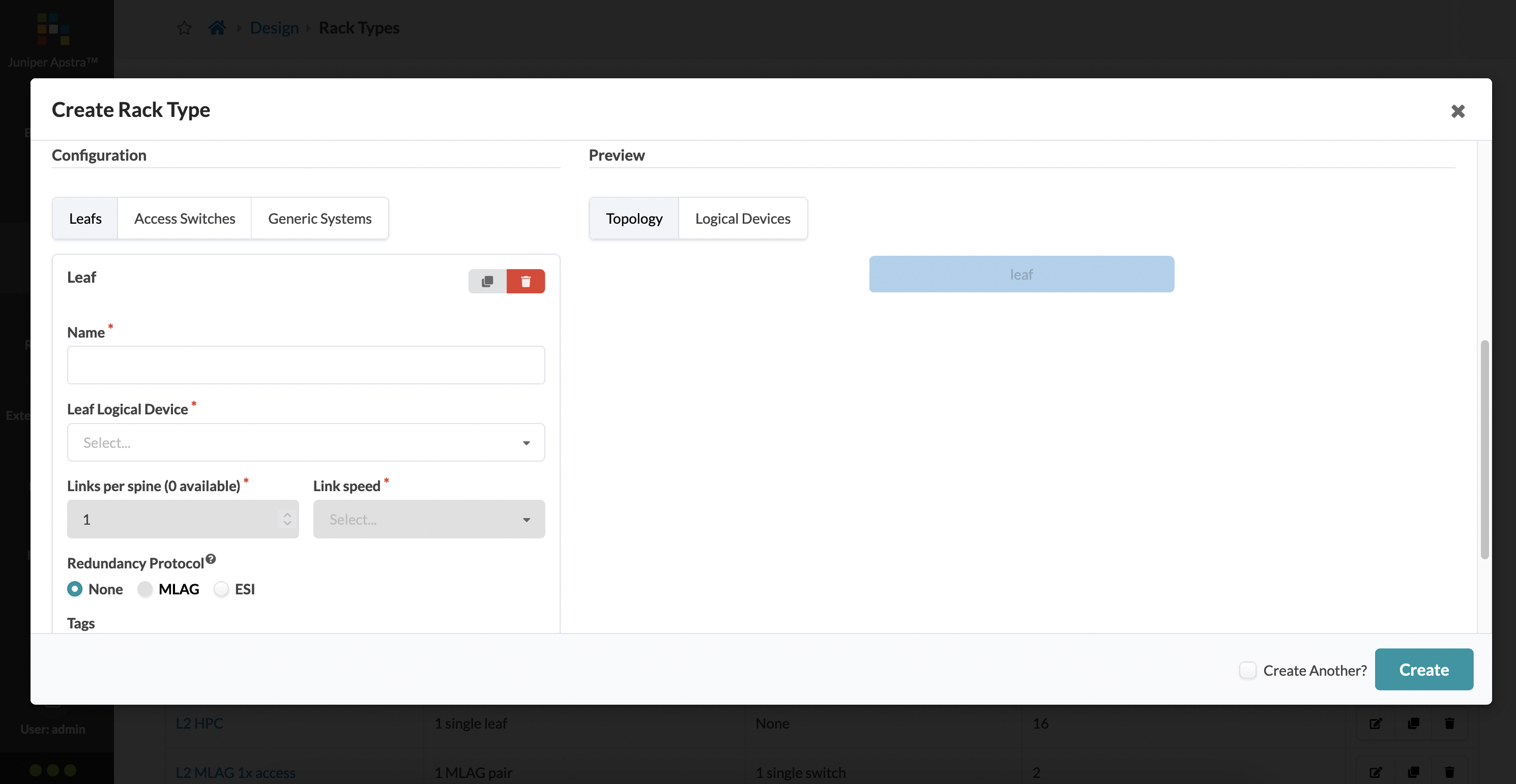
The main input for the leafs here are:

• a leaf logical device
• the redundancy model (none, MLAG or ESI)
• how many links per spine (these are taken from how many ports you’ve assigned as a connection to a spine)
• what kind of port speed for your spine facing links

Let’s provide these inputs for our rack:

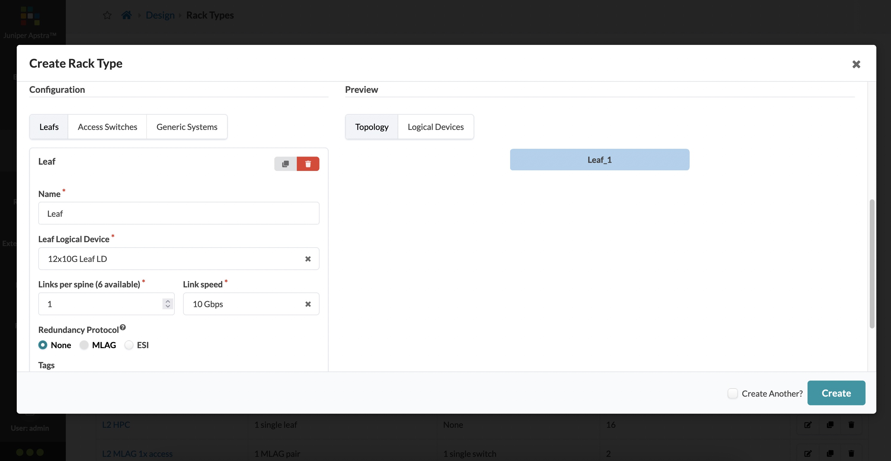
Because this is a one leaf rack, the redundacy model chosen is simply none. But watch what happens when you choose ESI:

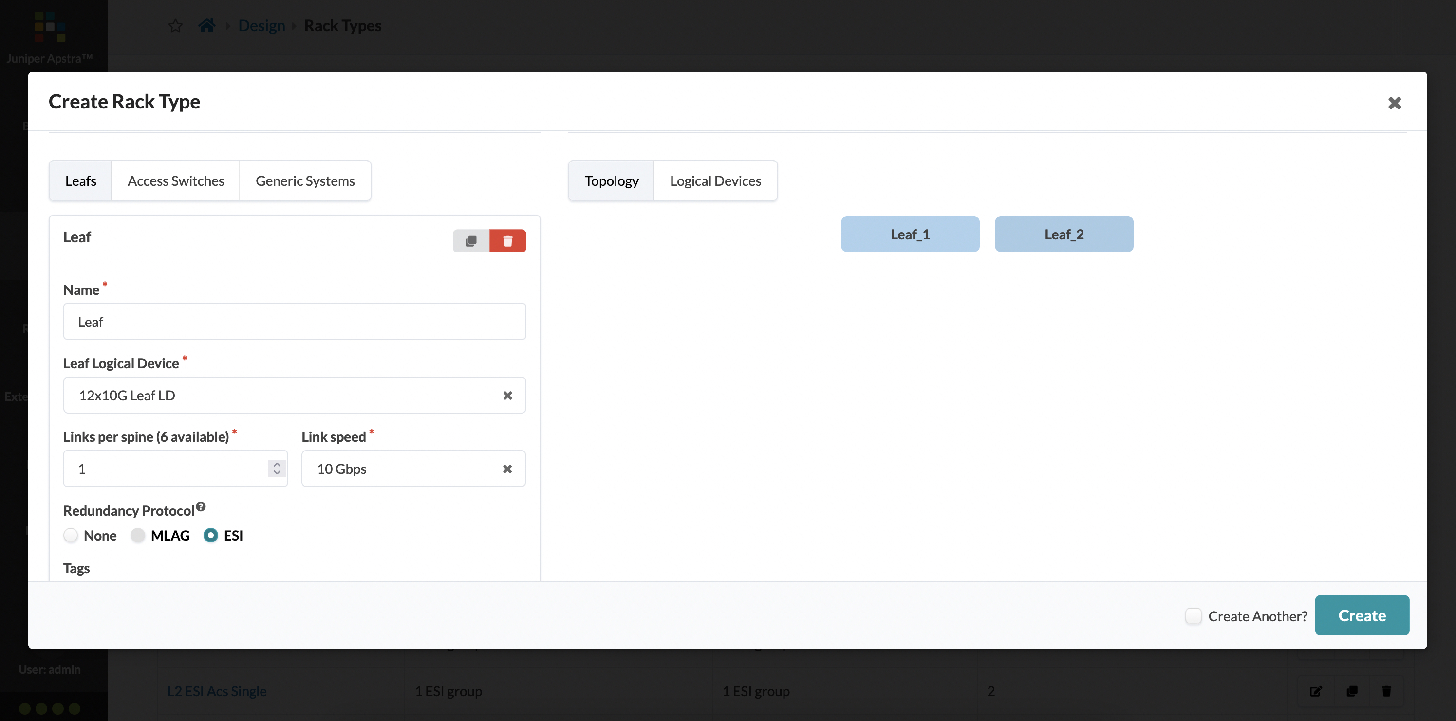
The number of leafs automatically becomes two. Any guesses on why MLAG is greyed out and cannot be selected? Go back to our logical device for this leaf - we never marked any ports that could be connected to another leaf, which naturally eliminates MLAG as an option since that requires a leaf to leaf connection.

Now that our leaf is defined, we need to declare the generic systems that will be present in the rack (and how they will be connected to the leaf).

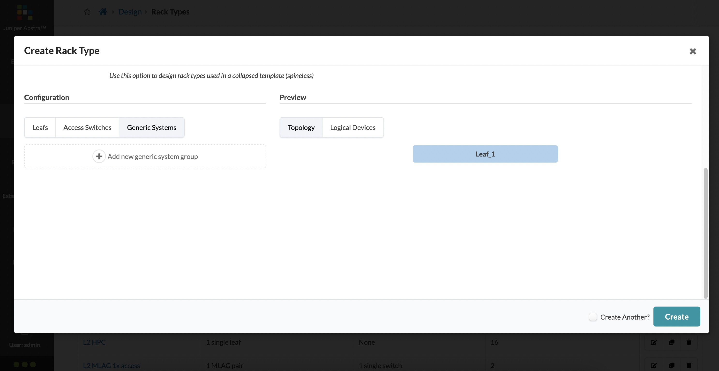
We’d like to have two hosts per rack, and each link is a 10G link back up to the leaf:

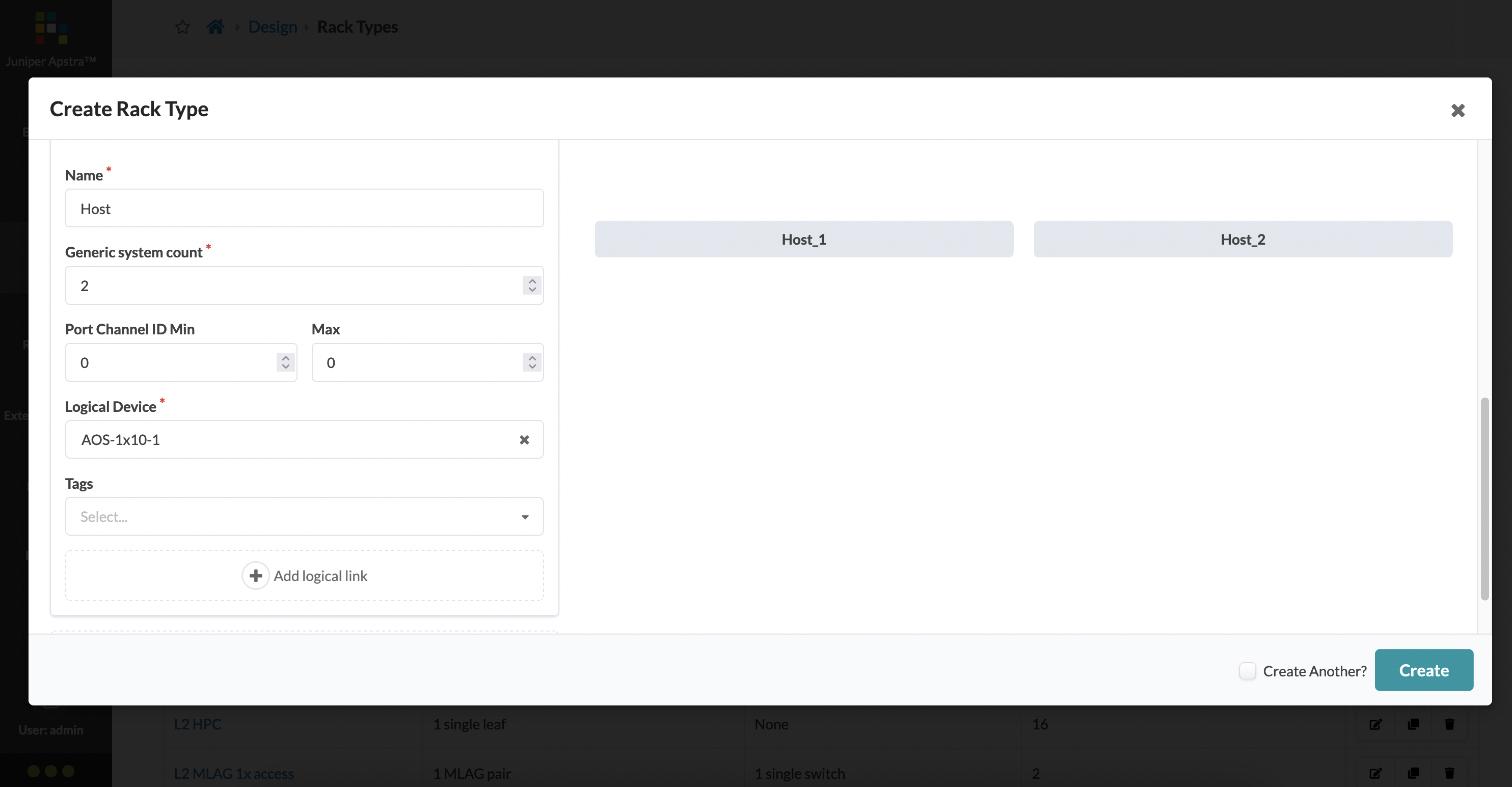
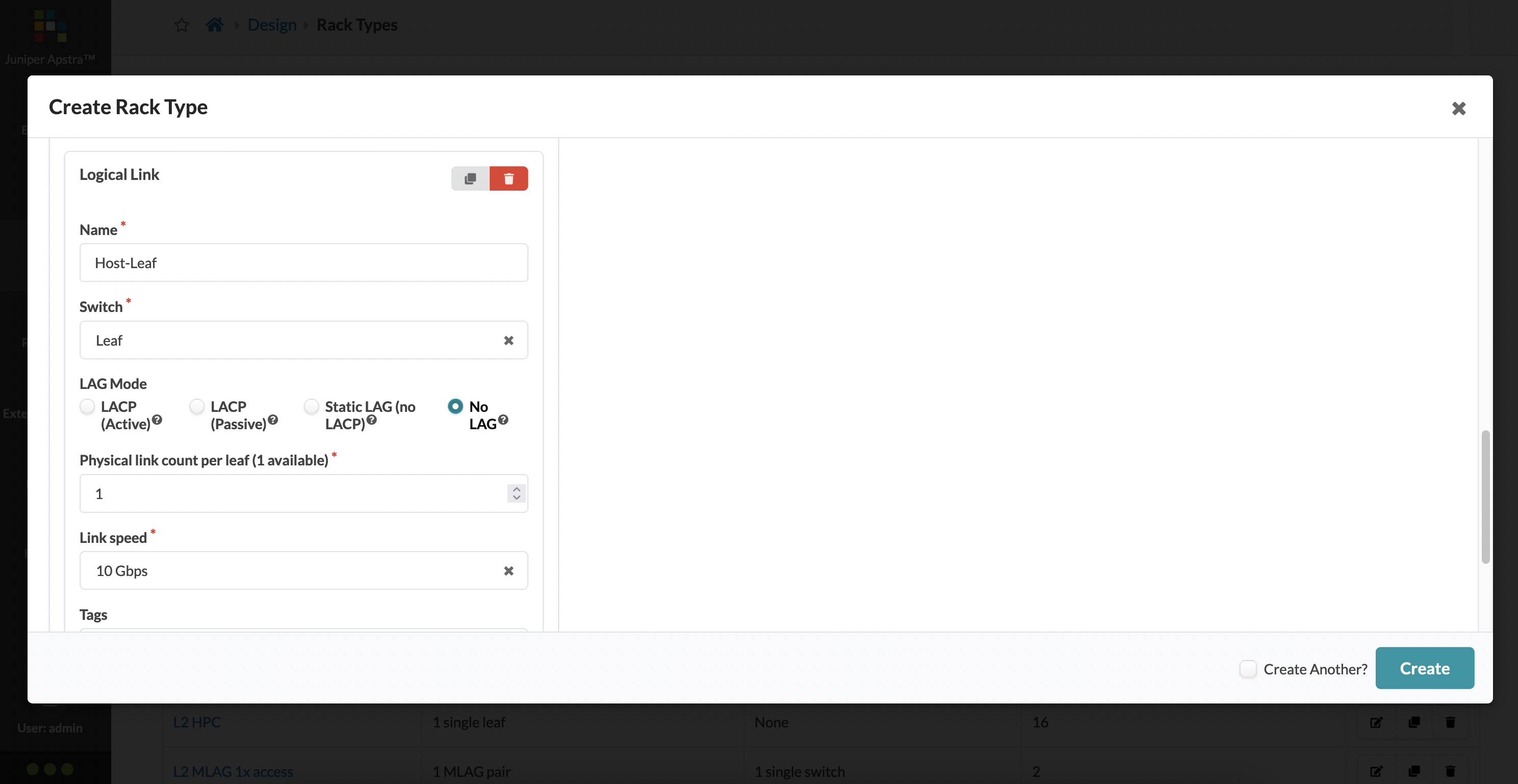
As part of the generic system definition, you need to also define properties of the link that will connect the host and the leaf. ‘Add logical link’ at the bottom allows you to do this. Here, you can configure how many links per host, if there is a need for LACP for link aggregation and so on.

And finally, you can click on ‘Create’ to create this rack. This is what it looks like visually:

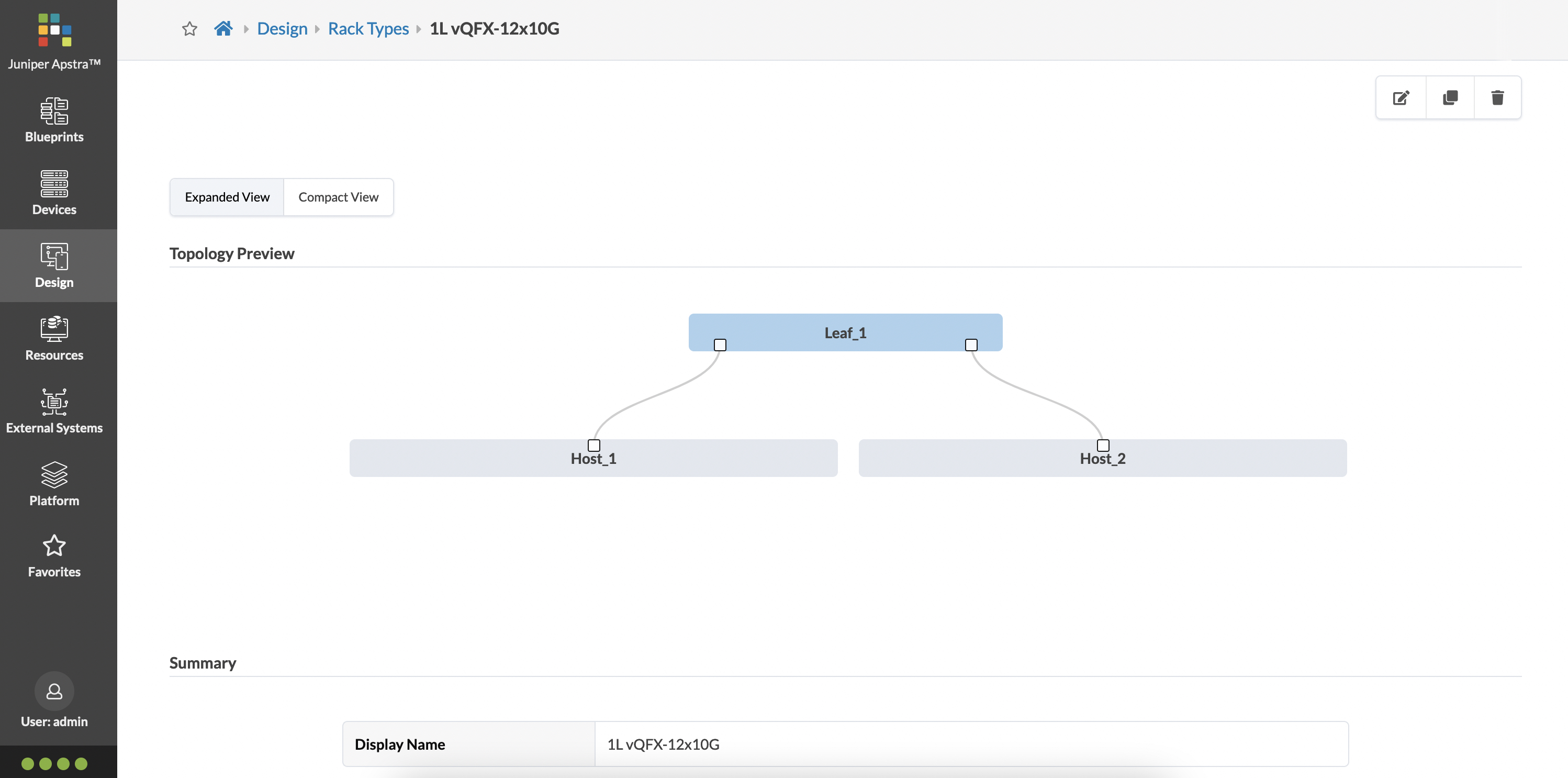
This visual representation of your rack is so cool! It shows you exactly what you built, what it looks like, and if you scroll further down, it shows you each element that was used to build this entire rack.

In the next post, we’re going to build a template, and then stage and deploy our data center.

References

1. Apstra 4.1 documentation